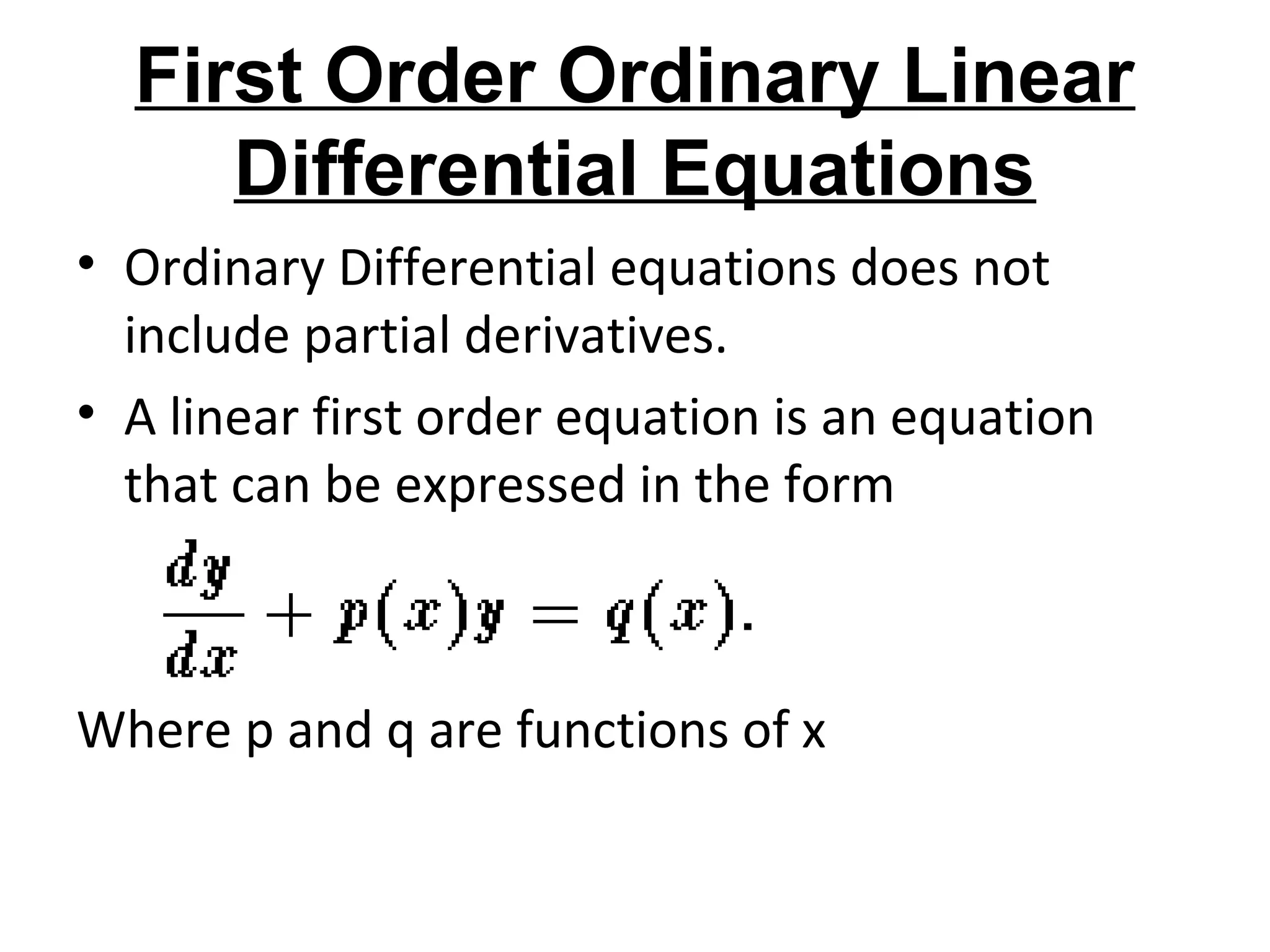
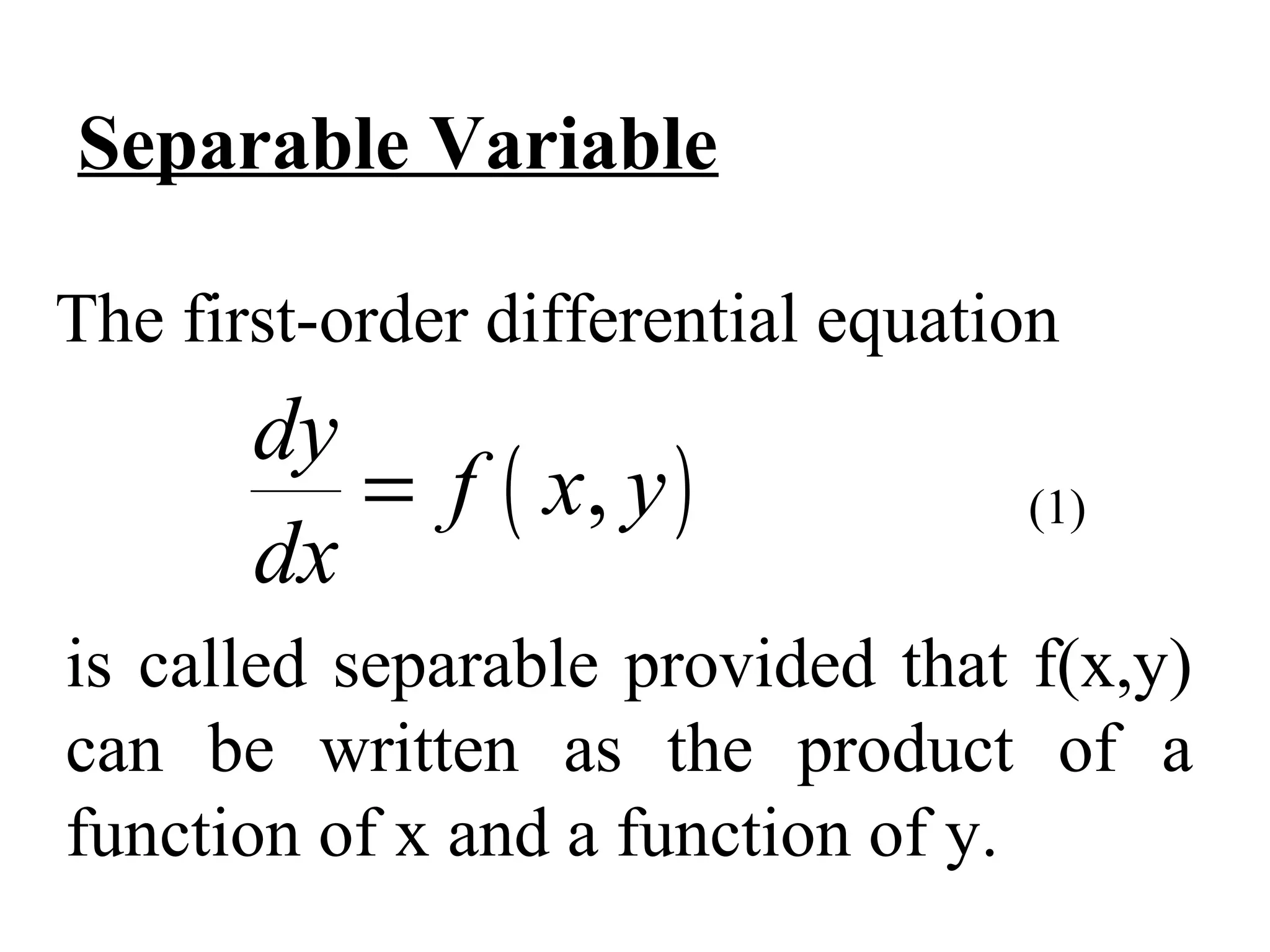
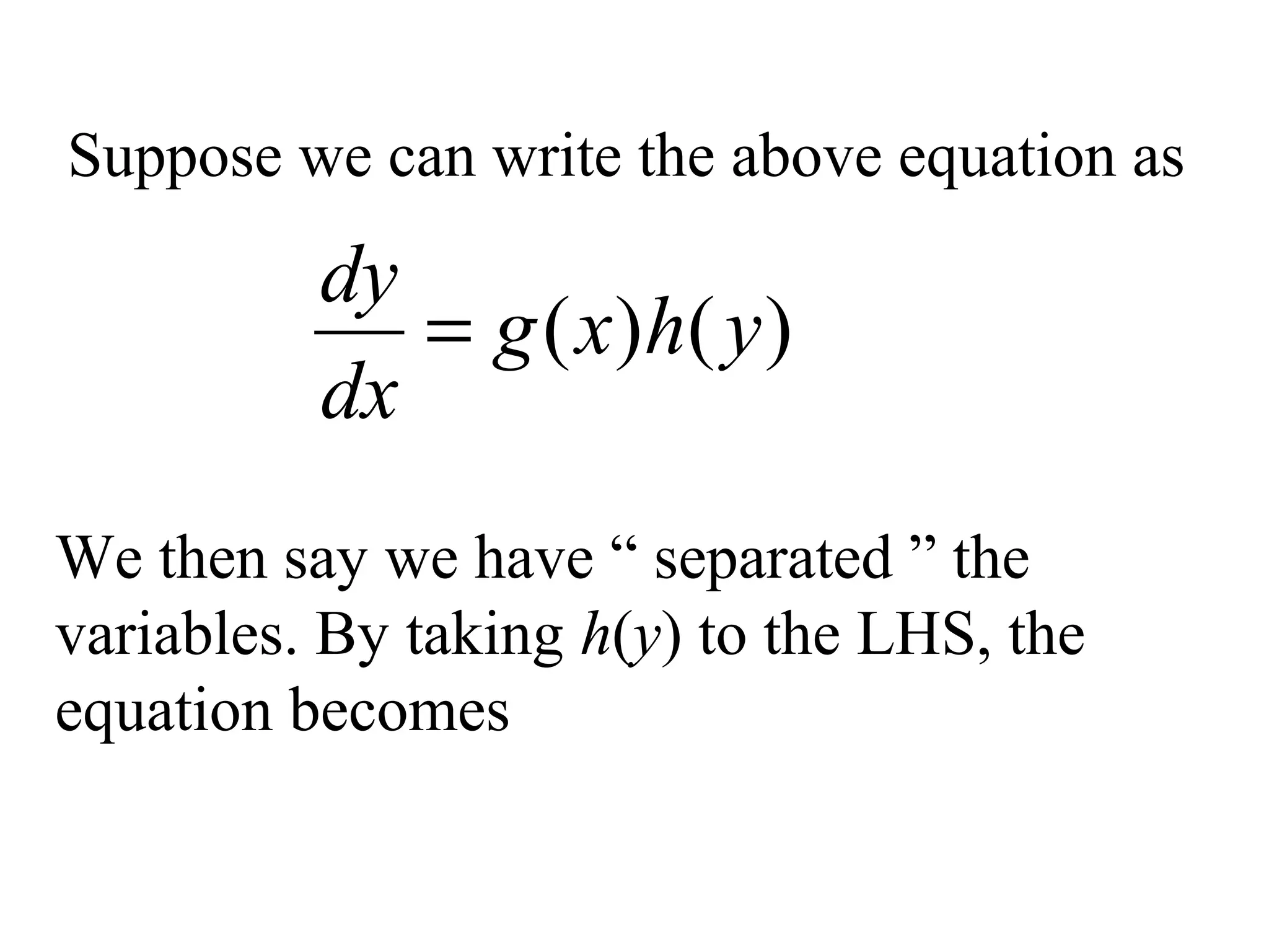
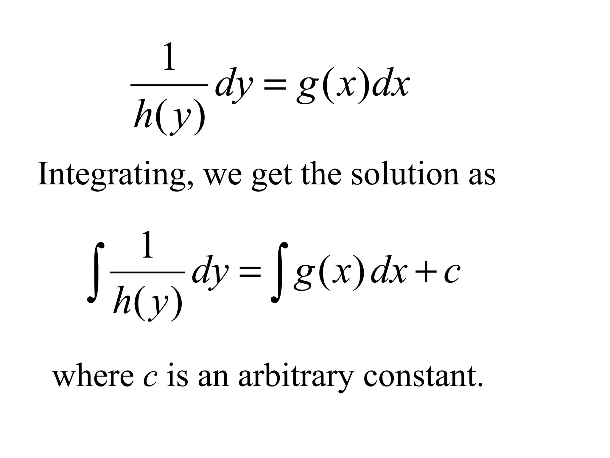
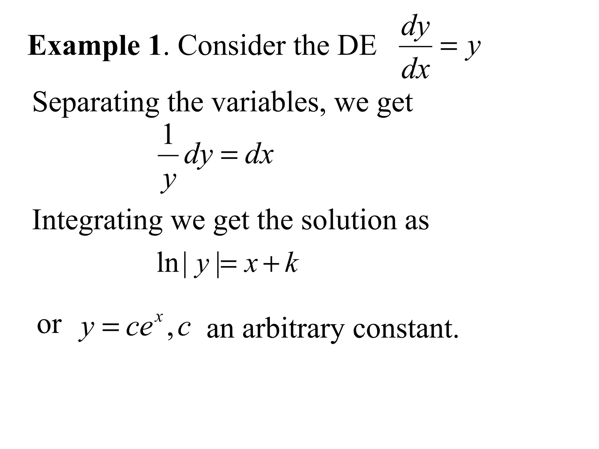
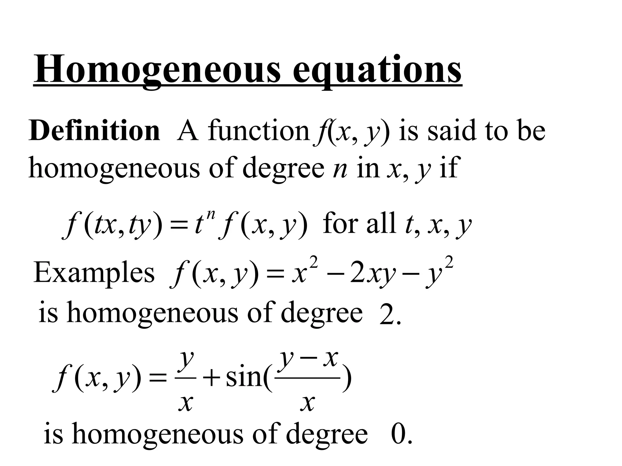
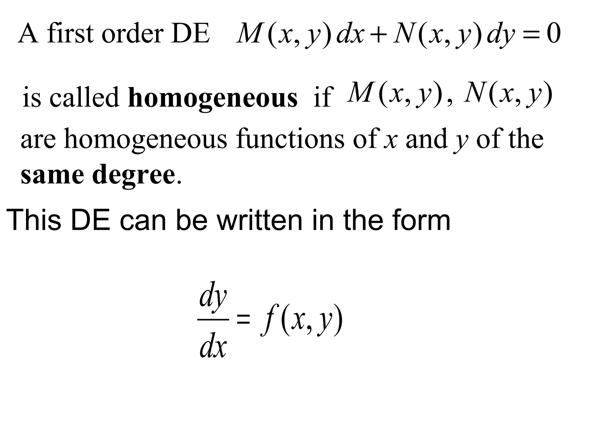
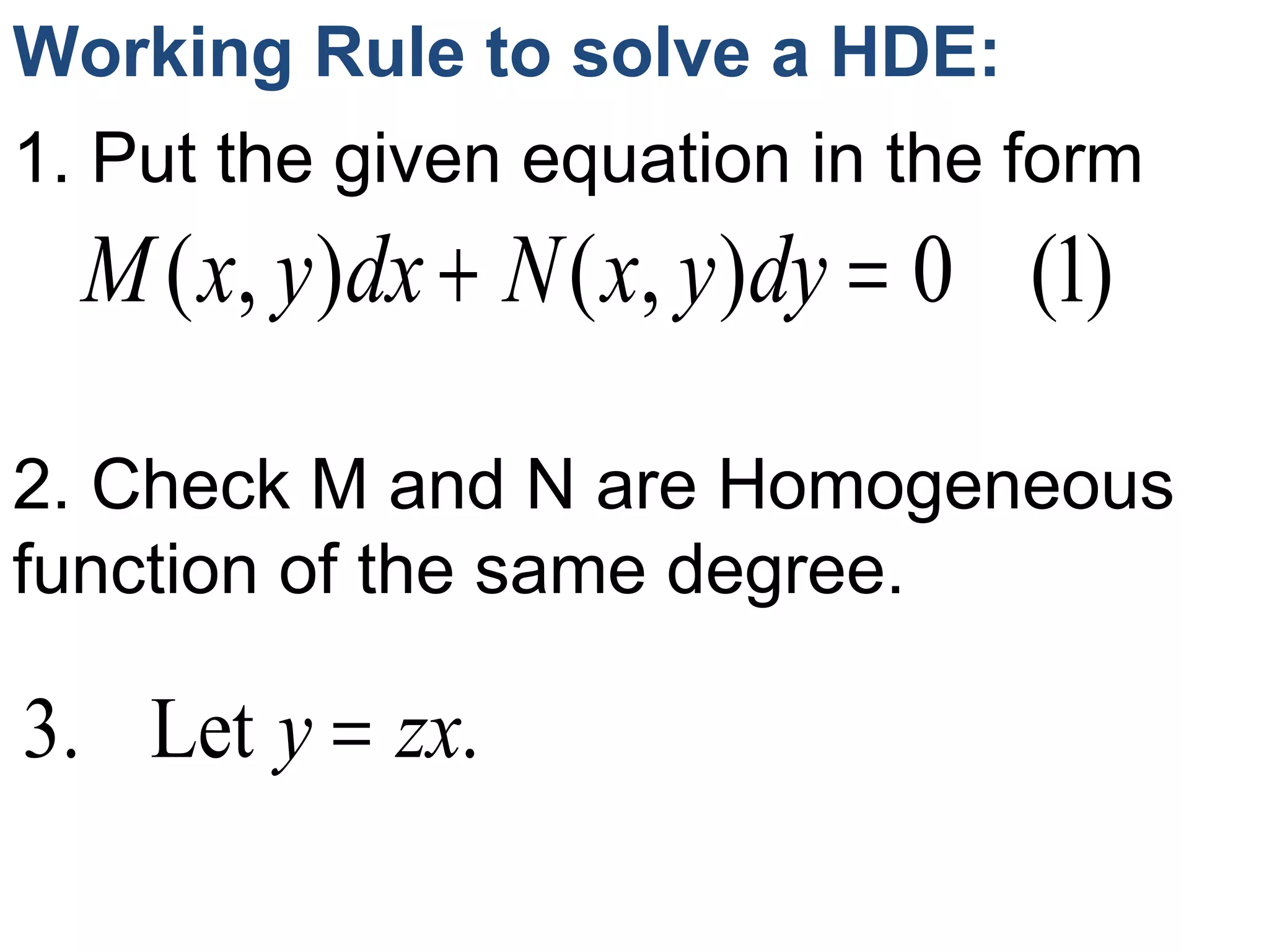
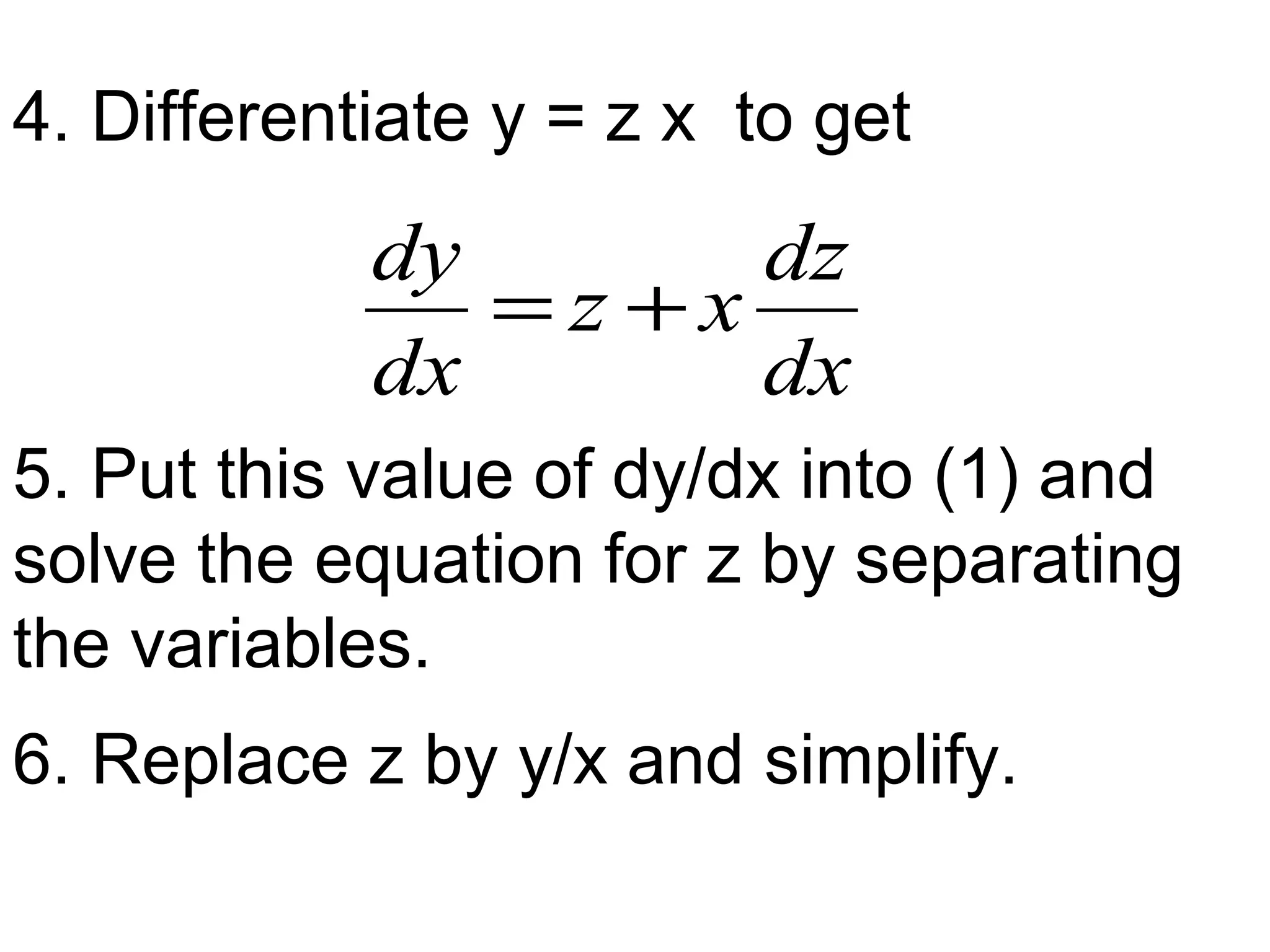
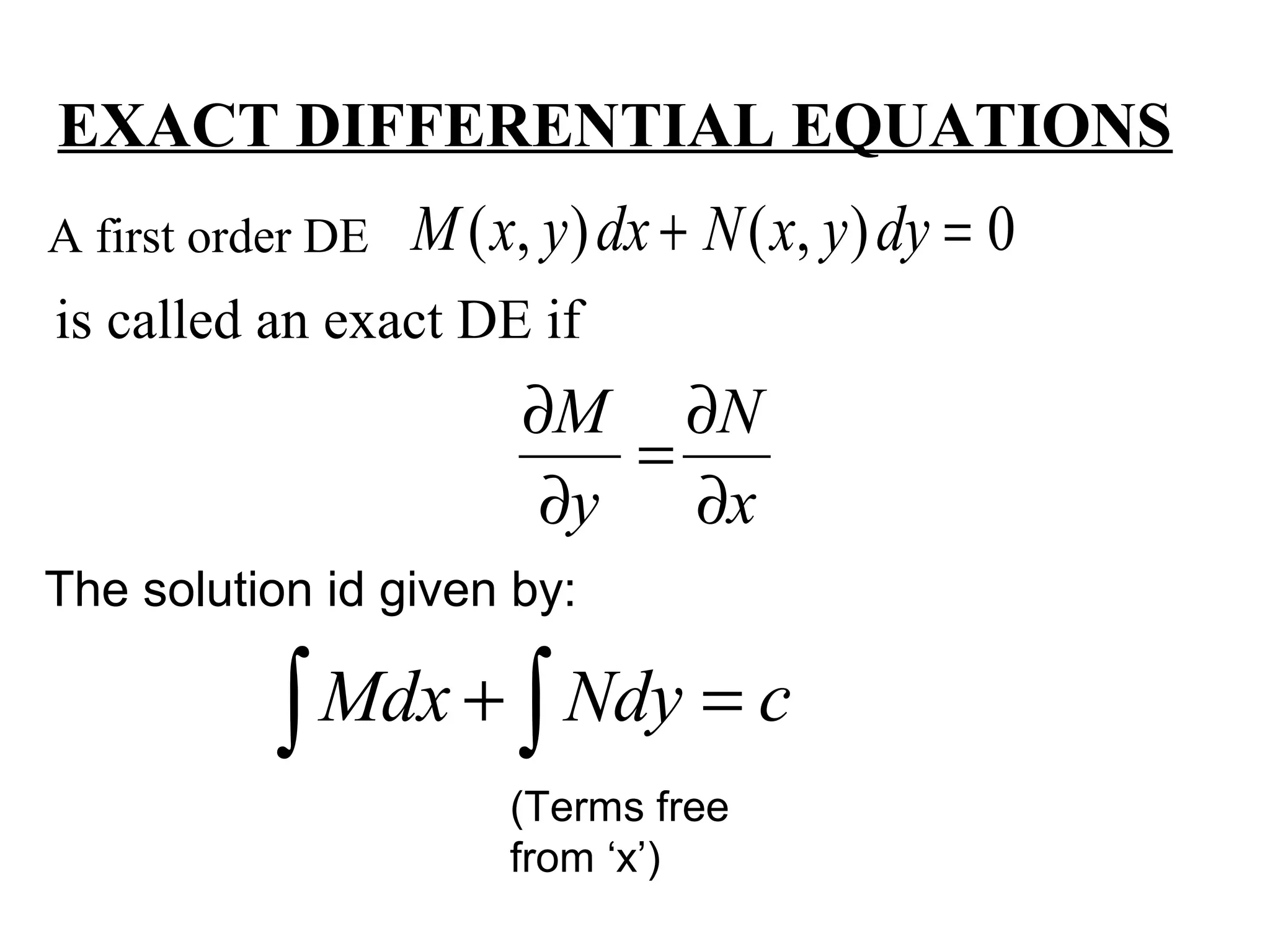
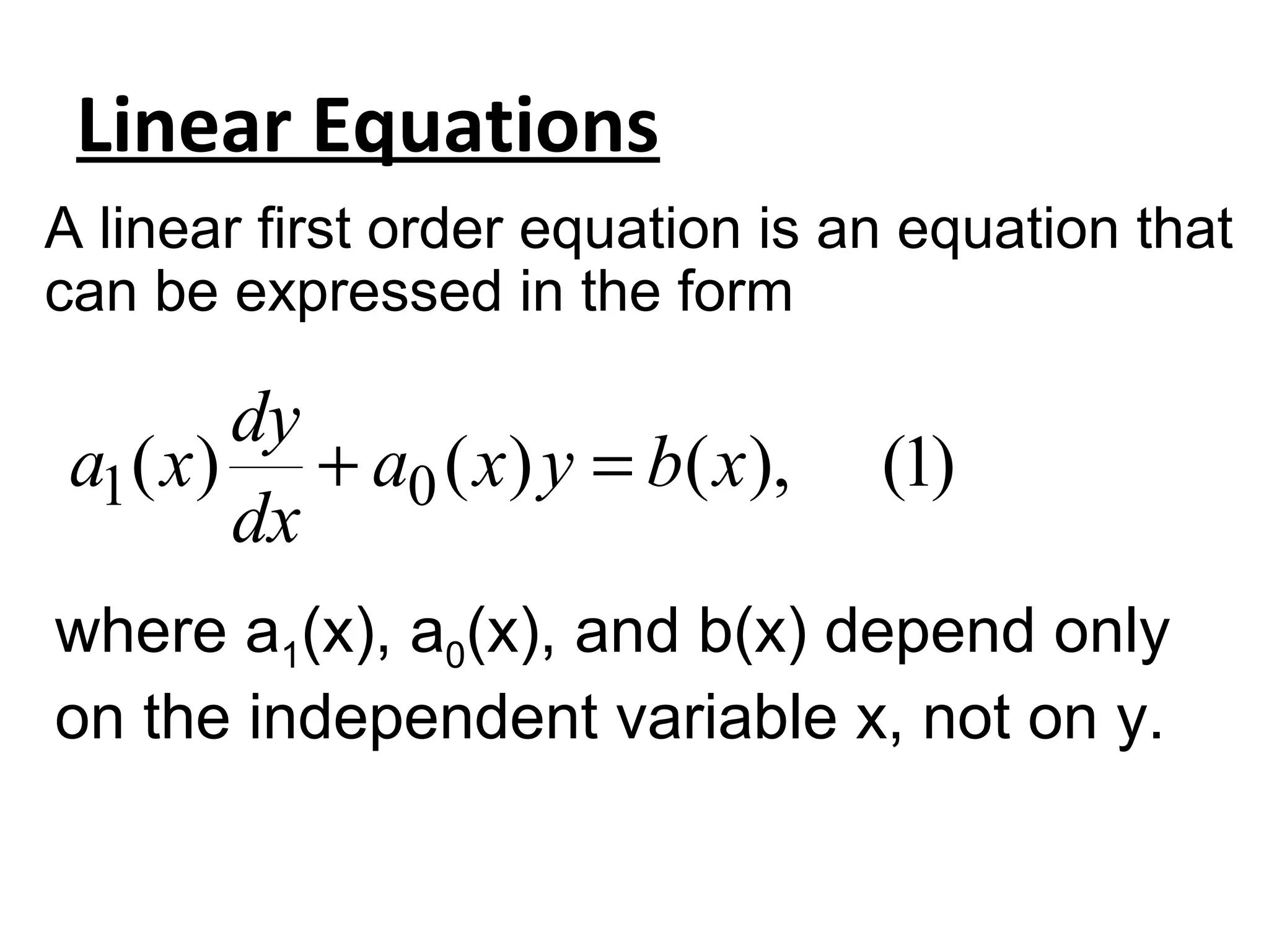
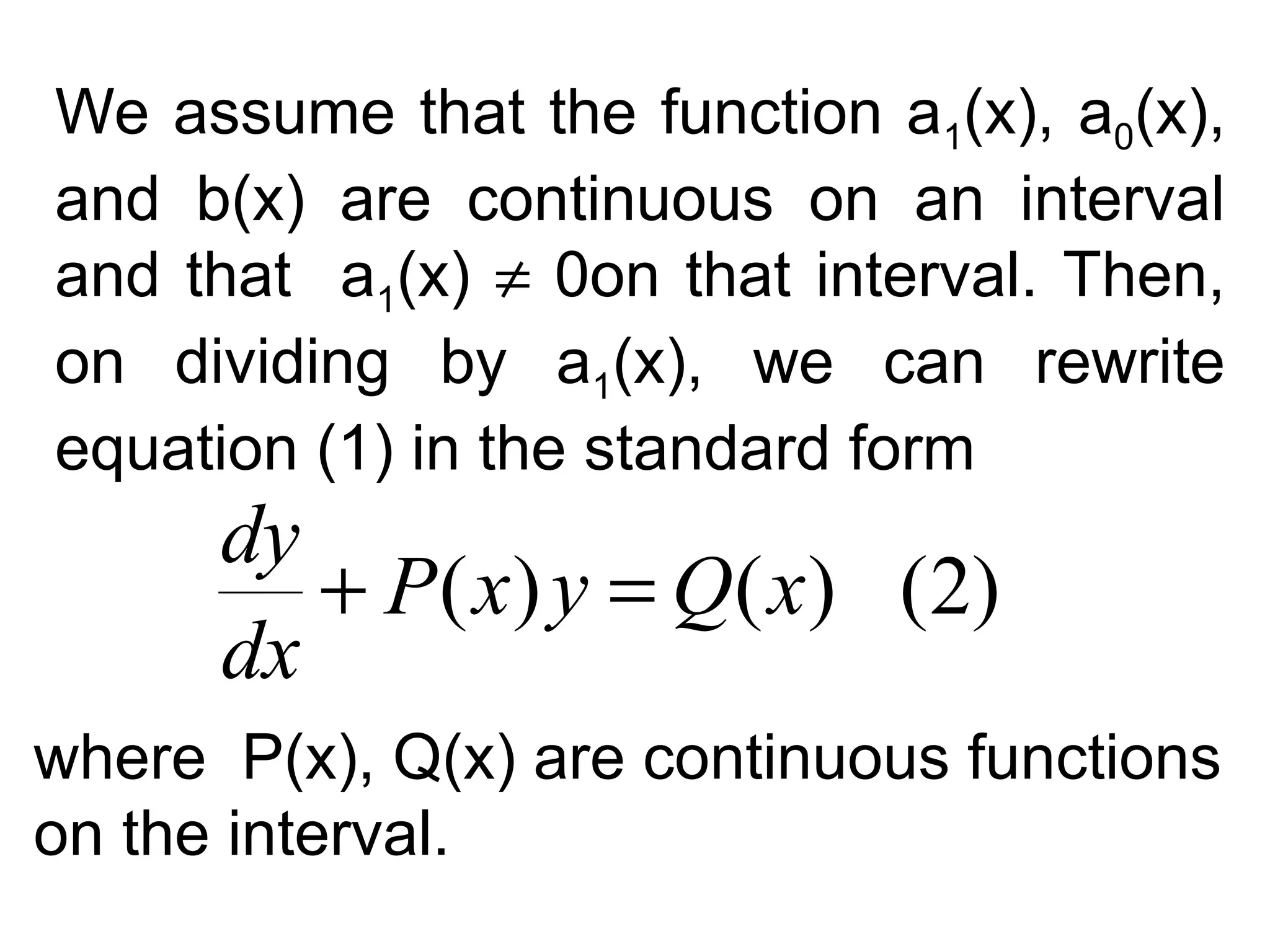
1) First order ordinary linear differential equations can be expressed in the form dy/dx = p(x)y + q(x), where p and q are functions of x. 2) There are several types of first order linear differential equations, including separable, homogeneous, exact, and linear equations. 3) Separable equations can be solved by separating the variables and integrating both sides. Homogeneous equations involve functions that are homogeneous of the same degree in x and y.

1. First Order Ordinary Linear
Differential Equations
• Ordinary Differential equations does not
include partial derivatives.
• A linear first order equation is an equation
that can be expressed in the form
Where p and q are functions of x

2. Types Of Linear DE:
1. Separable Variable
2. Homogeneous Equation
3. Exact Equation
4. Linear Equation

3. The first-order differential equation
( ),
dy
f x y
dx
=
is called separable provided that f(x,y)
can be written as the product of a
function of x and a function of y.
(1)
Separable Variable

4. Suppose we can write the above equation as
)()( yhxg
dx
dy
=
We then say we have “ separated ” the
variables. By taking h(y) to the LHS, the
equation becomes

5. 1
( )
( )
dy g x dx
h y
=
Integrating, we get the solution as
1
( )
( )
dy g x dx c
h y
= +∫ ∫
where c is an arbitrary constant.

6. Example 1. Consider the DE y
dx
dy
=
Separating the variables, we get
dxdy
y
=
1
Integrating we get the solution as
kxy +=||ln
or ccey x
,= an arbitrary constant.

7. Homogeneous equations
Definition A function f(x, y) is said to be
homogeneous of degree n in x, y if
),(),( yxfttytxf n
= for all t, x, y
Examples 22
2),( yxyxyxf −−=
is homogeneous of degree
)sin(),(
x
xy
x
y
yxf
−
+=
is homogeneous of degree
2.
0.

8. A first order DE 0),(),( =+ dyyxNdxyxM
is called homogeneous if ),(,),( yxNyxM
are homogeneous functions of x and y of the
same degree.
This DE can be written in the form
),( yxf
dx
dy
=

9. The substitution y = vx converts the given
equation into “variables separable” form and
hence can be solved. (Note that v is also a new
variable)

10. Working Rule to solve a HDE:
1. Put the given equation in the form
.Let.3 zxy =
)1(0),(),( =+ dyyxNdxyxM
2. Check M and N are Homogeneous
function of the same degree.

11. 5. Put this value of dy/dx into (1) and
solve the equation for z by separating
the variables.
6. Replace z by y/x and simplify.
dx
dz
xz
dx
dy
+=
4. Differentiate y = z x to get

12. EXACT DIFFERENTIAL EQUATIONS
A first order DE 0),(),( =+ dyyxNdxyxM
is called an exact DE if
M N
y x
∂ ∂
=
∂ ∂
The solution id given by:
∫ ∫ =+ cNdyMdx
(Terms free
from ‘x’)

13. Solution is:
cyxy
cdy
y
ydx
=+
=+∫ ∫
ln2
2
∫ ∫ =+ cNdyMdx

14. Integrating Factors
Definition: If on multiplying by µ(x, y), the DE
0M dx N dy+ =
becomes an exact DE, we say that µ(x, y)
is an Integrating Factor of the above DE
2 2
1 1 1
, ,
xy x y
are all integrating factors of
the non-exact DE 0y dx xdy− =

15. ( )
M N
y x
g x
N
∂ ∂
−
∂ ∂
=
( )g x dx
eµ ∫=
is an integrating factor of the given DE
0M dx N dy+ =
Rule 1: I.F is a function of ‘x’ alone.

16. Rule 2: I.F is a function of ‘y’ alone.
If , a function of y alone,
then
( )h y dy
eµ ∫=
is an integrating factor of the given DE.
x
N
y
M
∂
∂
−
∂
∂
M
( )yh=

17. is an integrating factor of the given DE
0M dx N dy+ =
Rule 3: Given DE is homogeneous.
µ=
+ NyMx
1

18. Rule 4: Equation is of the form of
( ) ( ) 021 =+ xdyxyfydxxyf
Then,
NyMx −
=
1
µ

19. Linear Equations
A linear first order equation is an equation that
can be expressed in the form
1 0( ) ( ) ( ), (1)
dy
a x a x y b x
dx
+ =
where a1(x), a0(x), and b(x) depend only
on the independent variable x, not on y.

20. We assume that the function a1(x), a0(x),
and b(x) are continuous on an interval
and that a1(x) ≠ 0on that interval. Then,
on dividing by a1(x), we can rewrite
equation (1) in the standard form
( ) ( ) (2)
dy
P x y Q x
dx
+ =
where P(x), Q(x) are continuous functions
on the interval.

21. Rules to solve a Linear DE:
1. Write the equation in the standard form
( ) ( )
dy
P x y Q x
dx
+ =
2. Calculate the IF µ(x) by the formula
( )( ) exp ( )x P x dxµ = ∫
3. Multiply the equation by µ(x).
4. Integrate the last equation.

22. Applications
)mTα(T
dt
dT
−=
αdt
)T(T
dT
m
=
−
•Cooling/Warming law
We have seen in Section 1.4 that the mathematical formulation of
Newton’s
empirical law of cooling of an object
in given by the linear first-order differential equation
This is a separable differential equation. We
have
or ln|T-Tm
|=αt+c1
or T(t) = Tm
+c2
eαt

23. In Series Circuits
i(t), is the solution of the differential equation.
)(tERi
dt
di
=+Ι
dt
dq
i =
)t(Eq
C
1
dt
dq
R =+
Si
nce
It can be
written as