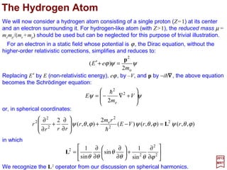
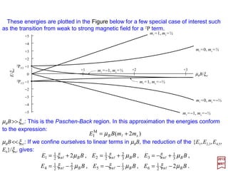
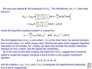
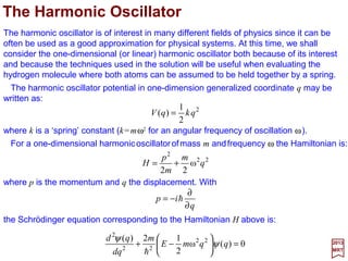
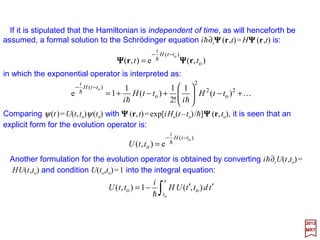
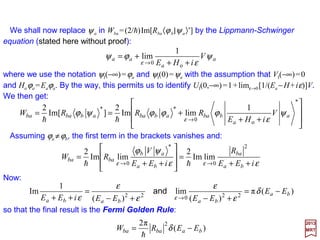
![Prolog
What you’re looking at is the first direct observation of an atom’s electron orbital — an atom’s actual wave
function! Up until this point, scientists have never been able to actually observe the wave function. Trying
to catch a glimpse of an atom’s exact position or the momentum of its lone electron has been like trying to
catch a swarm of flies with one hand. [c.f. Phys. Rev. Lett. 110, 213001 (2017)]
2](https://image.slidesharecdn.com/linked-inslides-hydrogen-130507131157-phpapp01/85/Part-V-The-Hydrogen-Atom-2-320.jpg)
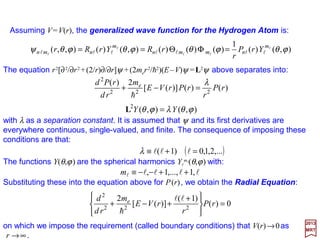
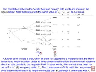
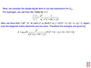
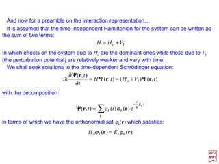
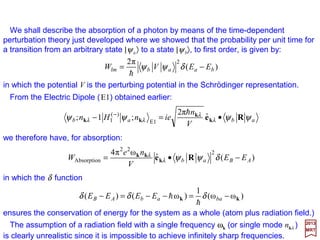
![Photoionization microscopy can directly obtain the nodal structure of the electronic orbital of a Hydrogen
atom placed in a static electric field. In the experiment, the Hydrogen atom is placed in the electric field E
and is excited by laser pulses. The ionized electron escapes from the atom and follows a particular tra-
jectory to the detector that is perpendicular to the field itself. Given that there are many such trajectories
that reach the same point on the detector, interference patterns can be observed […]. The interference
pattern directly reflects the nodal structure of the wavefunction. [c.f. Phys. Rev. Lett. 110, 213001 (2017)]
Calculated
Measured
3](https://image.slidesharecdn.com/linked-inslides-hydrogen-130507131157-phpapp01/85/Part-V-The-Hydrogen-Atom-3-320.jpg)
![with mo≡me the rest mass of the electron. By replacing E′ by E (non-relativistic energy);
eφ by −V,and p by −ih∇∇∇∇, the above equation becomes the static Schrödinger equation:
For an electron in a static field whose potential is ϕ, the Dirac equation (i.e., (E′+eϕ)ψ
={(1/2mo)[p+(e/c)A]2 +SMM[µS] Interaction−RE[p]−DT[p2]−SO[L••••S] Interaction}ψ – c.f.,
PART IV) without the higher-order relativistic corrections, simplifies and reduces to:
2017
MRT
ψψφ
o
2
2
)(
m
eE
p
=+′
in which the square of the angular momentum vector L is:
or, in spherical coordinates:
+=
+∇−= 22
e
22
e
2
)()()(
2
)( cmcEV
m
E prr ψψ
h
),,(),,()(
2
),,(
2 2
2
2
e
2
2
2
ϕθψϕθψϕθψ rrVE
rm
r
rrr
r L=−+
∂
∂
+
∂
∂
h
2
2
2
2
sin
1
sin
sin
1
ϕθθ
θ
θθ ∂
∂
+
∂
∂
∂
∂
=L
We recognize here the L2 operator from our discussion on spherical harmonics.
We will now consider a Hydrogen atom consisting of a single proton (Z=1) at its center
and an electron surrounding it. For hydrogen-like atoms (with Z>1), the reduced mass µ
=memp/(me +mp) should be used but can be neglected for this purpose of trivial illustration.
9](https://image.slidesharecdn.com/linked-inslides-hydrogen-130507131157-phpapp01/85/Part-V-The-Hydrogen-Atom-9-320.jpg)
(
2
22
e
2
2
ϕθλϕθ
λ
YY
rP
r
rPrVE
m
rd
rPd
=
=−+
L
h
lllll ,1,...,1, ++−−≡m
Substituting these into the equation above for P(r), we obtain the Radial Equation:
0)(
)1(
)]([
2
22
e
2
2
=
+
+−+ rP
r
rVE
m
rd
d ll
h
The equation r2[∂2/∂r2 +(2/r)∂/∂r]ψ +(2me r2/h2)(E−V )ψ =L2ψ above separates into:
),()(
1
)()()(),()(),,( ϕθϕθϕθϕθψ l
ll
l
l lllllll
m
nmmn
m
nmn YrP
r
rRYrRr =ΦΘ==
10](https://image.slidesharecdn.com/linked-inslides-hydrogen-130507131157-phpapp01/85/Part-V-The-Hydrogen-Atom-10-320.jpg)
![has solutions P(r)=exp(±ar) where a=√[−(2me/h2)E].
Solutions to this equation may be obtained by first considering the behavior at large r.
In the asymptotic region r →∞:
2017
MRT
)(e)(e)( o2
rfrfrP arra −−
==
where f (r) is a function to be determined by the Radial Equation and the boundary
conditions.
0)(
2)(
2
e
2
2
=+ rPE
m
rd
rPd
h
If E<0, exp(+ar)→∞ as r →∞. Since this violates (i.e., the ‘mathematical’ fact that the
exponential blows up at infinity!) the conditions (i.e., that it does not!) that the wave
function must be finite everywhere, it is not an acceptable solution (i.e.,itis not physically
possible!) On the other hand, exp(−ar)→0 as r →∞; it is therefore a possible solution.
If E >0, either sign in the exponent will satisfy the boundary conditions. We concentrate
on the case E<0, that is, the bound states of the atom.
The asymptotic behavior suggests that solutions to the Radial Equation be sought in
the form:
In the following slides, we will make use of the Bohr Radius (N.B., α =e2/hc=1/137):
11
( ) ( )MKSmorCGScm 11
2
e
2
o
o
8
e
2
e
2
o 1029.5
επ4
1052.0 −−
×==×===
em
a
cmem
a
hhh
α](https://image.slidesharecdn.com/linked-inslides-hydrogen-130507131157-phpapp01/85/Part-V-The-Hydrogen-Atom-11-320.jpg)
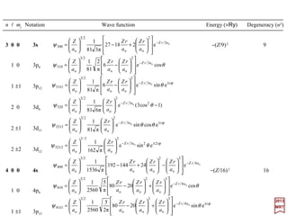
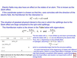
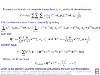
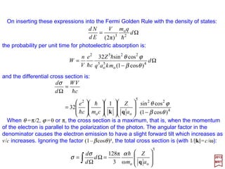
![0
5
10
ElectronVolt(eV)
13.60
n
1
2
3
4
5
∞ s p d f
LymanSeries
0
−5
−10
−13.60
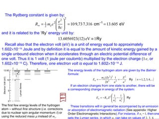
The first few energy levels of the Hydrogen
atom – without fine structure (i.e. corrections
due to nuclear spin angular momentum I ) or
using the reduced mass µ instead of me.
The energy levels of the Hydrogen atom are given by the
Balmer formula:
The Rydberg constant is given by:
and it is related to the ‘Ry’ energy unit by:
eV605.137.3169,7310
2
2
2
e2
1
==
= −
∞
1
cm
c
e
cmR
h
Ry1eV(12)13.6056923 ≡
Ry
−−= ∞ 2
1
2
2
2 11
nn
ZREn
( )...,4,3,2,1
1
2
)(
2
2
22
22
e
=−=−= n
n
Z
n
Zem
En Ry
h
If an electron changes from one state to another, there will be a
corresponding change in energy of the system:
These transitions will in general be accompanied by an emission
or absorption of electromagnetic radiation (c.f., Appendix: Higher
Order Electromagnetic Interactions). For instance, if n1 =1, then one
gets the Lyman series, in which n2 can take on values of 2, 3, 4, ….
Recall also that the electron volt [eV] is a unit of energy equal to approximately
1.602×10⁻¹⁹ J [Joule] and by definition it is equal to the amount of kinetic energy gained
by a single unbound electron when it accelerates through an electric potential difference
of one volt. Thus it is 1 Volt (1 Joule per Coulomb) multiplied by the electron charge (1e,
or 1.602×10⁻¹⁹ C [Coulomb]).Therefore,one electron volt is equal to: 1 eV =1.602×10⁻¹⁹ J.
2017
MRT
19](https://image.slidesharecdn.com/linked-inslides-hydrogen-130507131157-phpapp01/85/Part-V-The-Hydrogen-Atom-19-320.jpg)
,(),( 2* lll
lll =
Finally, the probability of finding an electron between ϕ and ϕ +dϕ is simply
proportional to dϕ.
20](https://image.slidesharecdn.com/linked-inslides-hydrogen-130507131157-phpapp01/85/Part-V-The-Hydrogen-Atom-20-320.jpg)
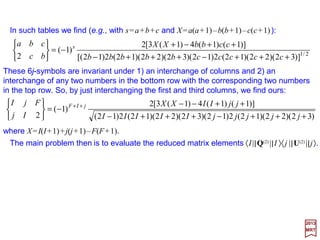
![Plot forY1
0,R10,and the probability densityψ100
∗ψ100=|ψ100|2 of the orbital [ yellow(+)/ blue
(−) on black] which is the probability of finding an electron around the atom’s nucleus.
2017
MRT
Plots for Y1
0 , R20, & |ψ200|2, Y1
0 , R21, & |ψ210|2, and for Y1
1 , R21, & |ψ211|2.
+½
−½
+½ −½
The maximum number
Nn of electrons in a
shell characterized by
principle number n is
given by twice (i.e. due
to spin) the number of
orbital stateswiththatn:
...,18,8,22
)12(2
2
1
0
==
+= ∑
−
=
n
N
n
n
l
l
21
+
−](https://image.slidesharecdn.com/linked-inslides-hydrogen-130507131157-phpapp01/85/Part-V-The-Hydrogen-Atom-21-320.jpg)
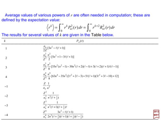
![Average values of various powers of r are often needed in computation; these are
defined by the expectation value:
2017
MRT
Expectation values 〈rk 〉 of rk for several values of k are given in the Table below.
∫∫
∞
+
∞
==
0
22
0
2
)()( drrRrdrrPrr n
k
n
kk
ll
〈rk〉
1
2
3
4
−1
−2
−3
−4
)]1(315[
2
2
2
2
2
o
+−+ lln
n
Z
a
k
)]1(3[
2
2o
+− lln
Z
a
)]1()1)(2(3)1)(2(30)1(35[
8
222
2
3
2
o
−+++−+−− llllllnnn
n
Z
a
]12)1033)(1(5)322(3563[
8
2224
4
4
4
o
+−+++−+− llllllnn
n
Z
a
2
o
1
na
Z
)½(
1
32
o
2
+lna
Z
lll )½)(1(
1
33
o
3
++na
Z
)½)(½)(1)((2
)1(3
2
35
2
4
o
4
−+++
+−
llll
ll
n
n
a
Z
24](https://image.slidesharecdn.com/linked-inslides-hydrogen-130507131157-phpapp01/85/Part-V-The-Hydrogen-Atom-24-320.jpg)
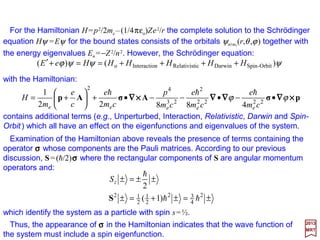
![For the Hamiltonian H=p2/2me −(1/4πεo)Ze2/r the complete solution to the Schrödinger
equation Hψ =Eψ for the bound states consists of the orbitals ψnlml
(r,θ,ϕ) together with
the energy eigenvalues En =−Z2/n2. However, the Schrödinger equation:
2017
MRT
with the Hamiltonian (see the Appendix – Higher Order Electromagnetic Interactions):
pAAp ××××∇∇∇∇ΣΣΣΣ∇∇∇∇∇∇∇∇××××∇∇∇∇ΣΣΣΣ ϕϕ •−•−−•+
+= 22
e
22
e
2
23
e
4
e
2
e 48822
1
cm
e
cm
e
cm
p
cm
e
c
e
m
H
hhh
ψψψϕ )()( Orbit-SpinDarwinicRelativistnInteractioo HHHHHHeE ++++==+′
contains additional terms (e.g., Unperturbed, Interaction, Relativistic, Darwin and Spin-
Orbit) which all have an effect on the eigenfunctions and eigenvalues of the system.
which identify the system as a particle with spin s=½.
±=±+=±
±±=±
222
¾)1½(½
½
hh
h
S
zS
Examination of the Hamiltonian above reveals the presence of terms containing the
operator ΣΣΣΣ whose components are the Pauli matrices, σσσσ =[σ1,σ2,σ3] (where σ1
REAL/SYM =
+1, σ2
COMPLEX/ANTI = mi, and σ3
REAL/DIAG
PARITY =±1). According to our previous discussion,
S =½hΣΣΣΣ where the rectangular components of S are angular momentum operators and:
Thus, the appearance of ΣΣΣΣ in the Hamiltonian indicates that the wave function of
the system must include a spin eigenfunction.
25](https://image.slidesharecdn.com/linked-inslides-hydrogen-130507131157-phpapp01/85/Part-V-The-Hydrogen-Atom-25-320.jpg)
![In the spin-½ [in units of h] case, we saw earlier that:
2017
MRT
=
=−=−
=
=+=+
=
−
+
χ
χ
1
0
½,½
0
1
½,½
, sms
The one-electron spin function is:
−=
+=
==
−
+
½
½
)(
s
s
sm
m
m
ms
for
for
χ
χ
ξξ
whereas the (one-electron) spin orbital is:
)()(),,,(),,( ssmmn mmmnr s
ξrξ ψψϕθψ == ll ll
It shall be understood that an integral involving spin orbitals implies a spatial integration
as well as a summation over spin coordinates. Also, we now have a degeneracy of 2n2
associated with the addition of spin eigenfunctionψnlmlms
(r,θ,ϕ,±½) andweuse |l,s;ml ,ms 〉
to identify the angular and spin parts of the wave function. Degenerate eigenfunctions
may be combined linearly to form other sets in a coupled representation of degenerate
eigenfunctions using the Clebsch-Gordan coefficients Cj
mlms
=〈l,s;ml,ms |l,s; j,mj 〉:
∑∑ ==
s
s
s mm
s
j
mm
mm
jssj mmsmjsmmsmmsmjs
l
l
l
lll lllll ,;,,;,,;,,;,,;, C
26](https://image.slidesharecdn.com/linked-inslides-hydrogen-130507131157-phpapp01/85/Part-V-The-Hydrogen-Atom-26-320.jpg)
![To see how this works out, let:
2017
MRT
or:
)( 222
2
1
SLJ −−=•SL
∫∫
∞∞
====
0
2
0
2
)()()()(,)(,)( rdrPrrdrrRrnrnr nnn lll ll ξξξξξ
3322
e
22
3322
e
22
1
2
,
1
,
2
)(
rrcm
eZ
n
r
n
rcm
eZ
r
h
ll
h
==ξ
Using the coupled representation:
The Hamiltonian HSO =ξ(r)L•S also contain the radial function ξ(r). So, to obtain the
energy corrections it is also necessary to evaluate the expectation value of ξ(r):
From the Table for 〈rk 〉 (with k=−3):
SLSLJSLJ •++== 2222
and++++
jjss
jjjj
ssjj
mjsSLJmjsmjsmjs
′′′+−+−+=
−−′′′′=•′′′′
δδδ llll
llll
)]1()1()1([
,;,,;,,;,,;,
2
1
222
2
1SL
In hydrogen, ξ(r) is given by ξ(r)=Ze2h2/2me
2c2r3 in which case:
lll )½)(1(
11
23
o
3
3
++
=
na
Z
r
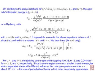
31](https://image.slidesharecdn.com/linked-inslides-hydrogen-130507131157-phpapp01/85/Part-V-The-Hydrogen-Atom-31-320.jpg)
![From the relation 〈l′,s′; j′,m′j|L•S|l,s;j,mj 〉=½[ j( j+1)−l(l+1)−s(s+1)]δl′lδs′sδj′j it is seen
that the matrix elements vanish unless:
These are the selection rules for spin-orbit coupling. Also, these are also valid:
0)(0 =+∆=∆=∆=∆ sj mmmj ll and
The Table below lists values of the 〈1,½; m′l,m′s|L•S|1,½;ml,ms 〉 matrix elements for p
states of ξnl= 〈n,l|ξ(r)|n,l〉 (and shortened to |ml ,ms 〉 since l=1 and s =½ for all states).
½,1−
2017
MRT
½,1
½,1 ½,0 ½,0 − ½,1− ½,1−−
½,1 −
½,0
½,0 −
½,1−
½,1 −−
2
1
2
1
−
2
1
2
1
0
0
2
1
2
1
2
1
−
2
1
1,01,0 ±=∆±=∆ smm andl
33](https://image.slidesharecdn.com/linked-inslides-hydrogen-130507131157-phpapp01/85/Part-V-The-Hydrogen-Atom-33-320.jpg)
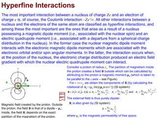
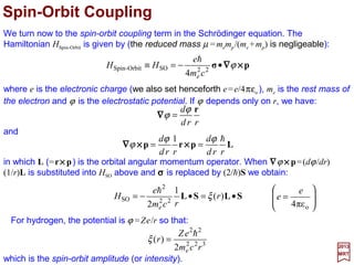
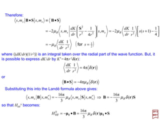
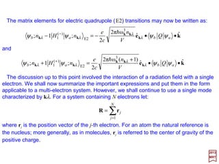
![The most important interaction between a nucleus of charge Ze and an electron of
charge e is, of course, the Coulomb interaction −Ze2/r. All other interactions between a
nucleus and the electrons of the same atom are classified as hyperfine interactions, and
among these the most important are the ones that arise as a result of a nucleus
possessing a magnetic dipole moment (i.e., associated with the nuclear spin) and an
electric quadrupole moment (i.e., associated with a departure from a spherical charge
distribution in the nucleus). In the former case the nuclear magnetic dipole moment
interacts with the electronic magnetic dipole moments which are associated with the
electronic orbital and/or spin angular momenta. In the latter, the interaction occurs when,
at the position of the nucleus, the electronic charge distribution produced an electric field
gradient with which the nuclear electric quadrupole moment can interact.
Magnetic field created by the proton. Outside
the proton, the field B is that of a dipole – µµµµI;
inside, the field Bi depends on the exact
partition of the magnetism of the proton.
5
22
o
5
o
5
o 3
π4
µ
3
π4
µ
3
π4
µˆˆˆ
r
rz
B
r
zy
B
r
zx
BBBB zyxzyx
−
===⇔++= IIIkjiB µµµ and,
The magnetic field inside the proton, Bi, is given by (SI system):
Consider a proton of radius ro. The partition of magnetism
inside the proton creates a field B outside which can be
calculated by attributing to the proton a magnetic moment µµµµI
(which is taken to be parallel to the z-axis – see Figure).
Hyperfine Interactions
z
y
x
B
µµµµI
Bi
3
o
o 2
π4
µ
r
Bi Iµ=
2017
MRT
where µo is the magnetic permeability of free space.
ro
The external field is thus purely dipolar.
For r >> ro, we obtain the components of B (by calculating the
rotational of AI = (µo/4π)[(µµµµI ×××× r)/r3]) (SI system):
51](https://image.slidesharecdn.com/linked-inslides-hydrogen-130507131157-phpapp01/85/Part-V-The-Hydrogen-Atom-51-320.jpg)
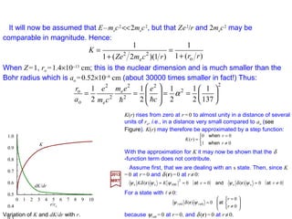
![To derive the form of this interaction we return to the Dirac equation(mo ≡me and q≡−e):
with:
2017
MRT
It is advantageous to separate the Hamiltonian into two parts:
where:
u
e
u )()(
2
1
)( ψψφ ππ ••=+′ ΣΣΣΣΣΣΣΣ K
m
eE
φecmE
cm
KcmEE
++′
=−=′ 2
e
2
e2
e
2
2
and
HFo
e2
1
HHe
c
e
K
c
e
m
H +=−
+•
+•= φApAp ΣΣΣΣΣΣΣΣ
φeKH −••= )()(o pp ΣΣΣΣΣΣΣΣ
HHF is the hyperfine Hamiltonian and it is the quantity we will be deriving.
u
e2
1
ψφψ
−
+•
+•=′ e
c
e
K
c
e
m
E ApAp ΣΣΣΣΣΣΣΣ
which becomes (with ππππ=p++++(e/c)A):
52
and:
)]()[(
2
)]()()()[(
2 2
e
2
e
HF AApAAp ••+••+••= ΣΣΣΣΣΣΣΣΣΣΣΣΣΣΣΣΣΣΣΣΣΣΣΣ K
cm
e
KK
cm
e
H](https://image.slidesharecdn.com/linked-inslides-hydrogen-130507131157-phpapp01/85/Part-V-The-Hydrogen-Atom-52-320.jpg)
![We concentrate on HHF which contains the entire dependence on the vector potential
A and the last term on the right is quadratic in A; it may therefore be neglected in a first
approximation.
2017
MRT
Also, since:
we have:
and HHF becomes:
)()(])()([)(()( r
r
rprrrrp f
rrd
dK
ifKKffKifKifΚ hhh −=+−=−= ∇∇∇∇∇∇∇∇∇)∇)∇)∇)
rrd
dK
K
r
=∇∇∇∇
rdr
dK
iKΚ
r
pp h−=
••+••−••= ))(())((
1
))((
2 e
HF pAArAp ΣΣΣΣΣΣΣΣΣΣΣΣΣΣΣΣΣΣΣΣΣΣΣΣ K
rdr
dK
iK
cm
e
H h
The potential φ is assumed to be a function of r only (i.e., φ(r)) which means that K
depends only on r (i.e., K(r)) so that:
Using the identity (ΣΣΣΣ•A)(ΣΣΣΣ•B)=A•B+iΣΣΣΣ•(A××××B), HHF is converted to:
)]([
1
)()(
2 e
HF ArArpAAppAAp ××××ΣΣΣΣ××××××××ΣΣΣΣ •+•−+•+•+•= i
rdr
dK
iKiK
cm
e
H h
53](https://image.slidesharecdn.com/linked-inslides-hydrogen-130507131157-phpapp01/85/Part-V-The-Hydrogen-Atom-53-320.jpg)
![With these relations, we get:
Finally:
2017
MRT
When these relations are included into our last development for HHF one obtains:
in which:
cm
e
B
e22
hh
== µandΣΣΣΣS
)(π4
3
)( 35
2
rµ
µr
rµ
µµµ
A δΙΙΙΙ
ΙΙΙΙ
ΙΙΙΙ
ΙΙΙΙΙΙΙΙΙΙΙΙ
++++−−−−∇∇∇∇∇∇∇∇××××∇∇∇∇××××∇∇∇∇××××∇∇∇∇
rrrrr
•=
∇−
•=
=
333
)(
])[(
1
][
1
rrrr
rµrµ
rµrµrrrµrAr ΙΙΙΙΙΙΙΙ
ΙΙΙΙΙΙΙΙΙΙΙΙ −−−−))))))))((((−−−−))))××××((((××××××××
•
=••==
••
+
•
+
•+
••
+
•
= 4253HF
))((
2)(π4
))((3)(
2
rrrd
dK
rr
KH BB
rSrµSµ
Sµr
rSrµSLµ II
I
II
µδµ
−−−−
with ΣΣΣΣ whose componentsare Pauli matricesσσσσ=[σ1,σ2,σ3]. We now examine K and dK/dr.
rZecmE
cm
K 22
e
2
e
2
2
++′
=
If ϕ is replaced by Ze/r, we have:
56](https://image.slidesharecdn.com/linked-inslides-hydrogen-130507131157-phpapp01/85/Part-V-The-Hydrogen-Atom-56-320.jpg)
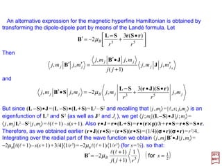
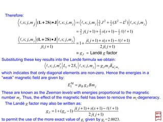
![An alternative expression for the magnetic hyperfine Hamiltonian is obtained by
transforming the dipole-dipole part by means of the Landé formula. Let
Then:
2017
MRT
and:
But since (L –S)•J=(L –S)•(L+S)=L2 −S2 and recalling that | j,mj〉=|l,s; j,mj 〉 is an
eigenfunction of L2 and S2 (as well as J2 and Jz ), we get 〈 j;mj|(L–S)•J| j;mj〉=
〈 j,mj|L2 −S2 | j,mj〉=l(l+1)−s(s+1). Also r•J=r•(L+S)=r•(r××××p)/h+r•S=r•S=S•r.
Therefore, as we obtained earlier (r•J)(r•S)=(r•S)(r•S)=(1/4)(ΣΣΣΣ•r)(ΣΣΣΣ•r)=r2/4.
Integrating over the radial part of the wave function we obtain 〈 j,mj |B′•J| j,mj〉=
−2µB[l(l+1)−s(s+1)+¾]〈1/r3〉=−2µBl(l+1)〈1/r3〉 (for s=½). so that:
•
+−=′ 53
)(3
2
rr
B
rSrSL
B
−−−−
µ
( )½
1
)1(
)1(
2 3
=
+
+
−=′ s
rjj
B for
ll
µB
sjj
jj
jj mjmj
jj
mjmj
mjmj ′
+
•′
=′′ ,,
)1(
,,
,, J
JB
B
jjBjj mj
rr
mjmjmj ,
))((3
,2,, 53
rSJrSL
SB
••
+−=•′
−−−−
µ
63](https://image.slidesharecdn.com/linked-inslides-hydrogen-130507131157-phpapp01/85/Part-V-The-Hydrogen-Atom-63-320.jpg)
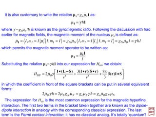
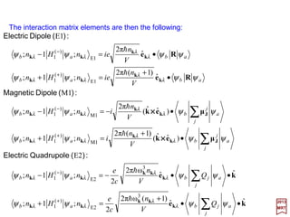
![For Hydrogen in an s state only the contact term is effective. Since l=0, J may be
replaced by S so that:
and, since the spin of the proton is I=½, we have also s=½ thus F=0 & 1. Hence:
which indicates that the only diagonal elements are non-zero. For the two possible
values of F, the energies are:
( )
( )
=−=−
==
=
0
4
3
π4
1
4
1
3
π4
2
100
2
100
FA
FA
E
FB
FB
ψγµ
ψγµ
h
h
)(
2
1 222
ISFSI −−=•
−+=
+−+−+=−−=•
2
3
)1(
2
1
)]1()1()1([
2
1
,)(½,,, 222
FF
IIssFFmFmFmFmF FFFF ISFSI
2S1/2
0.047 cm−1 (or 21 cm)
F = 1
F = 0
n = 1
Magnetic hyperfine splitting of the ground
state of hydrogen. The entire splitting is due
to the Fermi contact term geµBgNµN (i.e., a
quantum effect.).
o
2
100
3
61
3
6π1
a
AE B
FB
h
h
γµ
ψγµ ===∆
For hydrogen, |ψ 100|2 =1/πao
3 (ao =0.529×10⁻⁸ cm), γh =µN gN =
5.05×10⁻²³ erg/GHz and with µB =0.927×10⁻²⁰ erg/GHz, the
difference in energy between the two levels for E is:
2017
MRT
as show in the Figure. If we set ∆E= hν, the frequency ν is
1420.4058 MHz, which corresponds to a wavelength of 21 cm.
65](https://image.slidesharecdn.com/linked-inslides-hydrogen-130507131157-phpapp01/85/Part-V-The-Hydrogen-Atom-65-320.jpg)
![Next, we consider the dipole-dipole term in our last expression for HHF.
Also, we have I•J=½(F2 −I2 −J2) and 〈F,mF|I•J|F,mF〉=½[F(F+1)−I(I+1)− j( j+1].
Again, only the diagonal matrix elements are non-zero. Therefore the energies are given
by:
lll )½)(1(
11
33
o
3
3
++
=
na
Z
r
For hydrogen, we use from the Table for 〈rk〉:
)]1()1()1([
)½)(1(33
o
3
+−+−+
++
= IIjjFF
jjna
Z
E B
l
hγµ
2017
MRT
66](https://image.slidesharecdn.com/linked-inslides-hydrogen-130507131157-phpapp01/85/Part-V-The-Hydrogen-Atom-66-320.jpg)
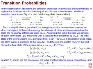
Yl
ml*(θ1,ϕ1)Yl
ml (θ2,ϕ2) – we get:
in which re is the position vector of the electron, rp is the position vector of the p-th
proton, and the sum is taken over all Z protons.
∑−=
=•=•
l
l
ll
llll
l
ll
m
mm
YY ),(),(),(),( eepp
*
ee
)(
pp
)()(
e
)(
p ϕθϕθϕθϕθ YYYY
∑
∞
=
+
>
<
•
+
=
0
1
)(
p
)(
e
pe
12
1
π4
1
l
l
l
ll
l r
r
YY
rr −−−−
Substitution in 1/|r1 −−−− r2|above yields:
z
y
x
rp re
|re − rp | e
Z eO
68](https://image.slidesharecdn.com/linked-inslides-hydrogen-130507131157-phpapp01/85/Part-V-The-Hydrogen-Atom-68-320.jpg)
![In such tables we find (e.g., with s=a+b+c and X=a(a+1)−b(b+1)−c(c+1)):
2017
MRT
where X=I(I+1)+ j( j+1)−F(F+1).
2/1
)]32)(22)(12(2)12)(32)(22)(12(2)12[(
)]1()1(4)1(3[2
)1(
2 +++−+++−
++−+
−=
cccccbbbbb
ccbbXX
bc
cba s
Themainproblemthen is to evaluatethe reduced matrix elements 〈I||Q(2)||I 〉〈 j ||U(2) || j〉.
These 6j-symbols are invariant under:
1) an interchange of columns and;
2) an interchange of any two numbers in the bottom row with the corresponding two
numbers in the top row.
)32)(22)(12(2)12)(32)(22)(12(2)12(
)]1()1(4)1(3[2
)1(
2 +++−+++−
++−−
−=
++
jjjjjIIIII
jjIIXX
Ij
FjI jIF
So, by just interchanging the first and third columns, we find ours:
71](https://image.slidesharecdn.com/linked-inslides-hydrogen-130507131157-phpapp01/85/Part-V-The-Hydrogen-Atom-71-320.jpg)
![The computation of 〈 j ||U(2) || j 〉 proceeds in analogous fashion. This time we define a
quantity eQ/2 as:
2017
MRT
where, from (i.e., for l=2) U(2) =−e√(4π/2⋅2+1)Ye
(2) /re
2+1, we get:
−
−=−= 5
e
2
e
2
e
3
e
ee
0
2
)2( 3
2
11
),(
5
π4
r
rz
e
r
YeUO ϕθ
We note that ∂2(−e/r)/∂z2 =−e(3z2 −r2)/r5 is the zz (diadic) component of the electric field
gradient tensor produced by an electron at a point whose coordinated with respect to the
electron are [x,y,z]. Since the origin of the coordinate system (see previous Figure) has
been positioned at the nucleus 2UO
(2) in the equation above is the zz component of the
electric field gradient tensor at the nucleus produced by an electron at re, or UO
(2) =
½(∂2V/∂z2)O =½Vzz where V is the potential due to the electron and the second derivative
is evaluated at the origin O (i.e.,at nucleus).We then have eq=〈 j,mj =j|Vzz | j,mj =j〉=〈Vzz〉
which is the average (or expectation value) of Vzz taken over the electronic state | j, j〉.
jmjUjmjQe jOj === ,,
2
1 )2(
qe
jj
jjjj
jj
)12(
)32)(32)(1)(12(
2
1)2(
−
++++
=U
Again, the use of the Wigner-Eckart theorem leads to the result:
73](https://image.slidesharecdn.com/linked-inslides-hydrogen-130507131157-phpapp01/85/Part-V-The-Hydrogen-Atom-73-320.jpg)
![Now (without proof – c.f. M. Weissbluth) assuming axial symmetry, Vxx =Vyy, we have:
2017
MRT
where Vzz =eq. For this case there are only diagonal elements with twofold degenerates
in mI, that is, states with ±mI have the same energy.
)]1(3[
)12(4
,,
)]3([
)12(4
2
2
QQ
22
Q
+−
−
==
−
−
=
IIm
II
qQe
mIHmIE
IIV
II
eQ
H
III
zzz
i. When I=1, the energies are:
( )
( )
=−
±=+
=−=+−
−
=
0
2
1
1
4
1
)23(
4
1
)]11(13[
)11.2(1.4 2
2
222
2
Q
I
I
II
mqQe
mqQe
mqQem
qQe
E
I = 1
mI EQ
(1/4)e2qQ±1
0 −(1/2)e2qQ
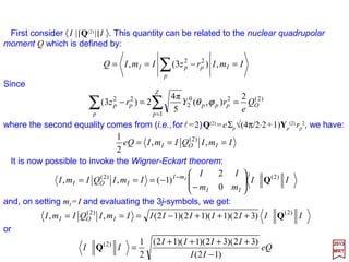
and the Figure below shows the quadrupole splitting (when I=1 and e2 qQ>0).
As has already been noted, the quadrupole interaction vanishes when I=0 or ½.
75](https://image.slidesharecdn.com/linked-inslides-hydrogen-130507131157-phpapp01/85/Part-V-The-Hydrogen-Atom-75-320.jpg)
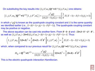
![ii. For I=3/2, the energies are:
2017
MRT
( )
( )
±=−
±=+
=
−=+−
−
=
2/1
4
1
2/3
4
1
4
15
3
12
1
)]12/3(2/33[
)12/3.2(2/3.4 2
2
222
2
Q
I
I
II
mqQe
mqQe
mqQem
qQe
E
and the Figure below shows the quadrupole splitting (when I=3/2 and e2 qQ>0).
and the Figure below shows the quadrupole splitting (when I=2 and e2 qQ<0).
I = 3/2
mI EQ
(1/4)e2qQ±3/2
−(1/4)e2qQ±1/2
I = 2
mI EQ
−(1/8)e2qQ±1
−(1/4)e2qQ0
(1/4)e2qQ±2
iii. Finally, for I=2, the energies are:
( )
( )
( )
=−
±=−
±=+
=−=+−
−
=
0
4
1
1
8
1
2
4
1
)63(
24
1
)]12(23[
)12.2(2.4
2
2
2
222
2
Q
I
I
I
II
mqQe
mqQe
mqQe
mqQem
qQe
E
76](https://image.slidesharecdn.com/linked-inslides-hydrogen-130507131157-phpapp01/85/Part-V-The-Hydrogen-Atom-76-320.jpg)
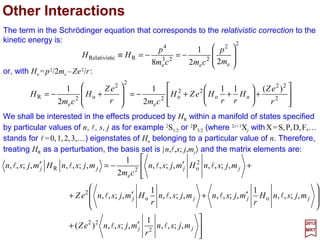
![This is the energy associated with the scalar potential energy, ϕ (105 cm−1).
And the significance of the various terms and their energies, is indicated to within an
order of magnitude (N.B., the ‘cm−1’ scale is given by the wave number 1/λ ≅ 8000 cm−1):
This contains the kinetic energy (i.e., p2 /2me) and interaction term (i.e., (e/2mec)(p • A+ A • p)
+ e2A2/2mec2) with a field represented by a potential vector A (105 cm−1). The interaction terms
are responsible or contribute to numerous physical processes among which are absorption,
emission and scattering of electromagnetic waves, diamagnetism, and the Zeeman effect.
2017
MRT
ϕe
The spin-orbit interaction (10-103 cm−1). More precisely, itis (eh/8mec2){σσσσ •[p −−−− (e/c)A]×××× E −−−−
σσσσ • E ×××× [p −−−− (e/c)A]} and it arises from the fact that the motion of the magnetic moment gives
rise to an electric moment for the particle which then interacts with the electric field.
This term appears in the expression of the relativistic energy:
and is therefore a relativistic correction to the kinetic energy (i.e., p2/2me) (0.1 cm−1).
The interaction of the spin magnetic moment (i.e., µS = 2⋅e/2me⋅h/2) with a magnetic field B=
∇∇∇∇ ×××× A (1 cm−1). Thus, it is the magnetic moment of one Bohr magneton, eh/2mec
(i.e., µB = 9.2741×10⁻²⁴ A⋅m2 or J/T) with the magnetic field.
2
e2
1
+ Ap
c
e
m
A××××∇∇∇∇σσσσ •
cm
e
e2
h
23
e
4
8 cm
p
L+−+≅+ 23
ee
2
2
e
2222
e
82
)(
cm
p
m
p
cmcpcm
4
ϕ∇∇∇∇∇∇∇∇ •− 22
e
2
8 cm
eh
This term produces an energy shift in s-states and is known as the Darwin (1887-1962) term
(< 0.1 cm−1). It is thus a correction to the direct point charge interaction due to the fact that in the
representation (Foldy-Wouthuysen), the particle is not concentrated at a point but is spread out
over a volume with radius whose magnitude is roughly that of a Compton wavelength, h/mec.
p××××∇∇∇∇σσσσ ϕ•− 22
e4 cm
eh
ϕe
c
e
m
−
+
2
e2
1
Ap
As a combination, this term represents the interaction of a point charge with the
electromagnetic field.
78](https://image.slidesharecdn.com/linked-inslides-hydrogen-130507131157-phpapp01/85/Part-V-The-Hydrogen-Atom-78-320.jpg)
![Eigenfunctions of the wave equation having different energy eigenvalues are
necessarily orthogonal, as we will now show. Let ψi and ψj be solutions of:
2017
MRT
If the integration is extended over all space, we obtain:
0)(
2 *
2
2
*2
2
*2
2
*2
2
2
2
2
2
2
*
=−+
∂
∂
+
∂
∂
+
∂
∂
−
∂
∂
+
∂
∂
+
∂
∂
∫ ∫ ∫
∫ ∫ ∫
∞
∞−
∞
∞−
∞
∞−
∞
∞−
∞
∞−
∞
∞−
zdydxdEE
m
zdydxd
zyxzyx
ijji
i
jjjiii
j
ψψ
ψ
ψψψψψψ
ψ
h
82
0)(
2
0)(
2 *
2
*2
2
2
=−+∇=−+∇ jjjiii VE
m
VE
m
ψψψψ
hh
and
Multiplying the terms in the first equation by ψ j
* and the terms in the second by ψi on the
right, and subtracting the second equation from the first, we obtain;
0)(
2
)( *
2
*22*
=−+∇−∇ ijjiijij EE
m
ψψψψψψ
h
or integrating over the particle coordinates after representing the system in Cartesian
coordinates, we obtain:
0)(
2
])([ *
2
*22*
=−+∇−∇ ∫∫ τψψτψψψψ dEE
m
d ijjiijij
h](https://image.slidesharecdn.com/linked-inslides-hydrogen-130507131157-phpapp01/85/Part-V-The-Hydrogen-Atom-82-320.jpg)
![Substituting V =V 0 +V ′, Ei =E0
i +E′i and ψi =ψ 0
i +ψ ′i into the Schrödinger equation
above and grouping the result in ascending order of approximation, we have:
2017
MRT
This first term is zero by comparing to the unperturbed Schrödinger equation, leaving us
with only the second term for a first-order approximation:
0])(-)()[()( 000000
=′′−′+′−+′−+− iiiiiiii EVEVEHEH ψψψψ assuchtermsordersecond
85
0)()( 000
=′−′+′− iiii EVEH ψψ
We now expand ψ ′i in terms of the complete orthonormal set of solutions to the
unperturbed Schrödinger equation, ψ 0
j. That is, we let:
∑
∞
=
=′
0
0
j
jjii a ψψ
which, with first-order approximation above, gives:
0)()( 0000
=′−′+−∑ ii
j
jjii EVaEH ψψ
Note that from H0ψ 0
i =E0
iψ 0
i, this last equation can be rewritten:
0)()( 0000
=′−′+−∑ ii
j
jjiij EVaEE ψψ
Multiplying this last equation by ψ 0
k
* on the left and integrating over all space, we get:
0)( 0*00*00*000
=′−′+− ∫∫∑ ∫ τψψτψψτψψ dEdVdaEE ikiik
j
jkjiij](https://image.slidesharecdn.com/linked-inslides-hydrogen-130507131157-phpapp01/85/Part-V-The-Hydrogen-Atom-85-320.jpg)
![The integrand in the last monster integral is essentially the electrostatic interaction
energy between two shells of charge density exp(−ρ1) and exp(−ρ2). To begin evaluating
it let us consider just the integral over ρ1. Let us consider further the potential at a point ρ
due to a shell of thickness dρ1 at ρ1; it is given by:
2017
MRT
and
)(eπ4
e
π4 111
1
12
1
1
1
ρρρρ
ρ
ρ
ρ ρ
ρ
<= −
−
ford
d
90
)(e
π4e
π4 11
2
1
12
1
1
1
ρρρρ
ρρ
ρ
ρ ρ
ρ
>= −
−
ford
d
)]2(e2[
π4
e
π4
eπ4)( 1
2
111
11
+−=+= −
∞
−
∞
−
∫∫ ρ
ρ
ρρ
ρ
ρρρφ ρ
ρ
ρ
ρ
ρ
dd
The total potential at ρ due to the infinite sphere of charge density exp(−ρ1) is given by:
This is the potential at a point ρ due to the entire distribution of charge density exp(−ρ1).](https://image.slidesharecdn.com/linked-inslides-hydrogen-130507131157-phpapp01/85/Part-V-The-Hydrogen-Atom-90-320.jpg)
![We can now evaluate the potential energy of interaction between the distribution of
charge density exp(−ρ1) and exp(−ρ2). The potential energy per unit volume of a charge
density exp(−ρ2) at a point ρ2 is given by (4πρ2)[2−(ρ2 +2)exp(−ρ2)]exp(−ρ2). Hence, the
second shell of charge 4πρ2
2exp(−ρ2)dρ2 has a potential energy of:
2017
MRT
91
])2(e2[
eπ)4(
2
2
2
2
2
2
2
2
+−
−
−
ρ
ρ
ρρ ρ
ρ
d
The total electrostatic potential of the sphere of charge density exp(−ρ2) due to the
sphere with charge density exp(−ρ1) is the integral over ρ2 of this last expression:
2
0
222
2
π)4(
4
5
])2(e2[eπ)4( 22
=+−∫
∞
−−
ρρρ ρρ
d
Therefore our monster integral yields a result of:
2
4
e
0
2
1
24
5
24
5
h
eZm
a
eZ
E ==′
and from Ei =−(meZ2e4/2h2)(1/n1
2 +1/n2
2)+ ∫ψ 1
0*
(1,0)ψ 2
0*
(1,0)(e2/r12)ψ 1
0
(1,0)ψ 2
0
(1,0)dτ above:
−−= ZZ
em
E
4
5
2
2
2
2
4
e
1
h
where mee4/2h2 is the ground state energy of the Hydrogen atom and 2Z 2 times this is
the unperturbed ground state energy of the two Helium electrons.](https://image.slidesharecdn.com/linked-inslides-hydrogen-130507131157-phpapp01/85/Part-V-The-Hydrogen-Atom-91-320.jpg)
![Consider a system of two identical particles such that one particle is in a state labeled
α and the other in another state labelled by β where α(1) represents particle 1 in state α,
&c. If particles 1 and 2 are interchangeable in either the α(1)α(2) or β(1)β(2) state, then
eigenfunction is unchanged and therefore these states are said to be symmetric. The
other states α(1)β(2) and β(1)α(2) are neither entirely symmetric nor entirely
antisymmetric, however, and it is convenient to treat them as a superposition of two
other states one of which is entirely symmetric and the other antisymmetric. We
therefore use linear combinations of the α(1)β(2) and β(1)α(2) states to represent the
two remaining wave functions of the system:
2017
MRT
where the factor 1/√2 is used for normalization. Since the α(1), β(2), α(2), and β(1) are
all solutions of the Schrödinger equation, the ψS and ψA will also be solutions. Now, in
our universe, systems of identical particles with integer spin must be represented by
wave functions which are symmetric with respect to the exchange of any two particles.
Similarly, all systems of identical particles with half-integer spin must be represented by
wave functions which are antisymmetric after exchange of any two particles. For multi-
electron system, this result was first postulated by W. Pauli in 1924 even before the
advent of quantum mechanics. The Pauli exclusion principle states that in a multi-elec-
tron atom there can never be more than one electron in the same quantum state. This
statement can be seen to be a consequence of saying that the electron wave function
must be antisymmetric since electrons belong to the half-integer class of particles.
)]2()1()2()1([
2
1
)]2()1()2()1([
2
1
αββαψαββαψ −=+= AS or
94](https://image.slidesharecdn.com/linked-inslides-hydrogen-130507131157-phpapp01/85/Part-V-The-Hydrogen-Atom-94-320.jpg)
![Towards the end of the The Hydrogen Atom chapter we saw that the wave function for
an electron with spin could be written as follows:
2017
MRT
so that for the Helium atom with two electrons we will have to take the appropriate
combination of the two wave functions ψa(1)=ψa(1)ξξξξa and ψb(2)=ψb(2)ξξξξb, where ψa(1)
represents the first electron at position 1 with a spin z-component represented by ξξξξa (i.e.,
either +½h or −½h) and similarly for ψb(2). The total wave function for the two electrons
will have to be the appropriate combination of space and spin states that makes it
antisymmetric. This total wave function can of course be written as the product of a
space part times a spin part; if the space part is symmetric, the spin part must be
antisymmetric and vice versa. As we have seen, the space part can be written:
95
smmn ξξ llψψψ == SpinSpace
_ _ _
_
)]1()2()2()1([
2
1
)]1()2()2()1([
2
1
babaAbabaS ψψψψψψψψψψ −=+= or](https://image.slidesharecdn.com/linked-inslides-hydrogen-130507131157-phpapp01/85/Part-V-The-Hydrogen-Atom-95-320.jpg)
![The spin wave function will be a bit more complicated because the separate spin
angular momenta can add vectorially just as the orbital and spin angular momenta do in
the case of the two-electron atom. Instead of having J=L+S, here S=s1 ++++s2 so that S=0
or 1. The magnitude of S will of course be √[S(S+1)]h.
2017
MRT
For S=0, ms =0 and we have just a single state while for S=1, ms =+1, 0, −1 and a triplet
spin state results. This corresponds to the three possible orientations with respect to
some preferred (i.e., z) direction in space and is equivalent to saying that we can start
with the following four spin combinations: ξξξξa(½)ξξξξb(½), ξξξξa(−½)ξξξξb(−½), ξξξξa(½)ξξξξb(−½), and
ξξξξa(−½)ξξξξb(½) to construct four symmetric and antisymmetric combinations:
tripletsymmetric
singletricantisymmet
-
)½()½(
)]½()½()½()½([
2
1
)½()½(
1
0
1
1
1
1
-)]½()½()½()½([
2
1
00
−−
−+−
−
+
−−−
ba
baba
ba
baba
smS
ξξ
ξξξξ
ξξ
ξξξξ
96](https://image.slidesharecdn.com/linked-inslides-hydrogen-130507131157-phpapp01/85/Part-V-The-Hydrogen-Atom-96-320.jpg)
![The total eigenfunction must be antisymmetric and thus we can form the following
combination from ψS , ψA and the above four spin combinations:
2017
MRT
and
97
]-[]-[ tripletsymmetricandsingletricantisymmet ⊗⊗ AS ψψ
or:
)]½()½()½()½([)]1()2()2()1([
2
1
babababa ξξξξ −−−⊗+ ψψψψ
−−
−+−⊗−
)½()½(
)]½()½()½()½([
2
1
)½()½(
)]1()2()2()1([
2
1
ba
baba
ba
baba
ξξ
ξξξξ
ξξ
ψψψψ
Notice that if the spin part of the wave function is symmetric, corresponding to parallel
spins, the space part must be antisymmetric. This has the interesting and important
consequence that the electrons will have small probability of being found close together
if they have parallel spins and a maximum probability of being found close together if
they have antiparallel spins. One can say that in effect parallel spins repel and
antiparallel spins attract.](https://image.slidesharecdn.com/linked-inslides-hydrogen-130507131157-phpapp01/85/Part-V-The-Hydrogen-Atom-97-320.jpg)
![By use of these matrix elements between the various hydrogen-like wave functions,
the secular determinant is written as:
2017
MRT
since all the Js and Ks with the same subscript are equal.
0
)(000000
)(000000
00)(0000
00)(0000
0000)(00
0000)(00
000000)(
000000)(
pp
pp
pp
pp
pp
pp
ss
ss
=
∆−
∆−
∆−
∆−
∆−
∆−
∆−
∆−
EJK
KEJ
EJK
KEJ
EJK
KEJ
EJK
KEJ
105
where ∆E is the small energy shift due to the perturbation. This determinant can be
rewritten as:
0])][()[( 32
p
2
p
2
s
2
s =−−∆−−∆ KJEKJE](https://image.slidesharecdn.com/linked-inslides-hydrogen-130507131157-phpapp01/85/Part-V-The-Hydrogen-Atom-105-320.jpg)
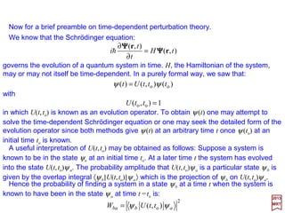
![x
y
x
y
r
ψ0
S
ψ0
A
ψ0
S
ψ0
A
r
When r is large the electron can be thought of as belonging to one proton or the other,
but as r becomes small this distinction is not possible and we must consider the effects
of exchange degeneracy. In this case, we ought then to take the total wave function as
being either symmetric or antisymmetric. For convenience we take both protons to be
lying on the x-axis so that under an exchange it is only the x coordinate that varies. Then
we write:
2017
MRT
Further, for the ground state U100 we choose the x-axis so that we have U100(x,0,0). Both
ψ0
S and ψ0
A are shown in the Figure for different values of r. Looking at these plots, we
see that as r→0 (at x=0), ψ0
S →maximum and ψ0
A →0.
)],,(),,([
2
1
)],,(),,([
2
1
2121 zyxUzyxUzyxUzyxU nn
A
nnn
S
n −=+= ψψ or
120
Illustrating the form of the symmetric and antisymmetric wave functions of the H2
++++ molecule for two
different proton separation distances (Left vs Right) .](https://image.slidesharecdn.com/linked-inslides-hydrogen-130507131157-phpapp01/85/Part-V-The-Hydrogen-Atom-120-320.jpg)
![Then the degenerate perturbation integrals are:
2017
MRT
and
∫∫ ′= 212B1A2
*
B1
*
A )()()()( ττψψψψ ddHJ rrrr
127
where dτ1 and dτ2 are the differential spherical volume elements (e.g., dτ1 =
r1
2sinθ1dr1dθ1dϕ1). The second term in the exchange integral K with H0, which we will
label K0, must be included because our initial wave functions are not orthonormal. Since:
∫∫∫∫ +′= 211B2A
0
2
*
B1
*
A211B2A2
*
B1
*
A )()()()()()()()( ττψψψψττψψψψ ddHddHK rrrrrrrr
)()(2)()()()( 1B2A11B2A
0
1B2A
0
rrrrrr ψψψψψψ EEH ==
we have:
∫∫= 211B2A2
*
B1
*
A10 )()()()(2 ττψψψψ ddEK rrrr
The contribution of e2/rAB term to J is simply e2/rAB, since the wave functions are
normalized and e2/rAB may be taken outside the integration over the electron
coordinates. Similarly, the contribution of the e2/rAB term to K is simply [(e2/rAB)/2E1]K0.
The contribution of e2/r1B to J would be ∫ψA
*(r1)(−e2/r1B)ψA(r1)dτ1 since ψB(r2) is
normalized and r1B is not a function of the position of the second electron. The
contribution of e2/r1B to K would be similar.](https://image.slidesharecdn.com/linked-inslides-hydrogen-130507131157-phpapp01/85/Part-V-The-Hydrogen-Atom-127-320.jpg)
![It is found that the symmetric wave function:
2017
MRT
is the correct zero-order wave function which with its antisymmetric twin causes the
perturbation matrix to be diagonal. The wave function above is also the symmetric wave
function whose eigenvalue is approximately E0 −K, the lower of the two energy
eigenvalues including resonances. This is in contrast to the case of Helium where both
electrons are in the same atom, and the antisymmetric wave function was found to be
the lower of the two energy eigenvalues including resonances. The attractive bonding
force of the Hydrogen molecule has been shown to be due to the possibility of two
electrons being in a symmetric state (i.e., being interchangeable in the space wave
function representation). Since no more than two electrons can be in one symmetric
state at the same time, the degeneracy in this case can be only twofold.
)]()()()([
2
1
1B2A2B1A
1
0
rrrr ψψψψψ +
+
=
E
K
S
129](https://image.slidesharecdn.com/linked-inslides-hydrogen-130507131157-phpapp01/85/Part-V-The-Hydrogen-Atom-129-320.jpg)
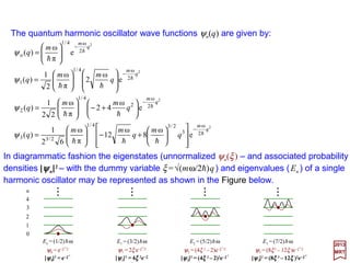
![The eigenfunctions of the harmonic oscillator version of the Schrödinger equation:
in which Hn(x) is a Hermit polynomial* of degree n and the eigenvalues are:
2017
MRT
A more convenient form to the ψn(q) solution above is achieved by changing the
variables to:
We then have:
which has the properties:
nn
m
uq
m
q ψξ
ω
ω
)(
h
h
== and
)()1()(
22
1
1
2
1
2
1
11
11
ξξξ
ξ
ξ
ξ
ξδξ
n
n
nnnn
nnnnnmnm
uuu
n
u
n
u
unu
d
d
unu
d
d
duu
−=−+
+
=
+=
−=
+=
−+
+−
∞+
∞−∫
and
,,,
=
−
q
m
H
m
n
q n
q
m
nn
hh
h ω
e
π
ω
!2
1
)(
2
2
ω4/1
2/
ψ
( ),...,,nnEn 210ω)½()ω( =+= h
* The Hermit polynomials are solutions to the differential equation d2Hn/dx2 – 2xdHn/dx − 2nHn = 0 and have a solution of the form
Hn(x) = (−1)n exp(x2)dn[exp(−x2)]/dxn. The first four Hermit polynomials are H0(x) = 1, H1(x) = 2x, H2(x) = −2 + 4x2 and H3(x)= −12x + 8x3.
)(e
)!2π(
1
)( 2
2/12/
2
ξξ ξ
nnn H
n
u −
=
142](https://image.slidesharecdn.com/linked-inslides-hydrogen-130507131157-phpapp01/85/Part-V-The-Hydrogen-Atom-142-320.jpg)
![We shall now investigate the harmonic oscillator be means of a matrix formulation. For
convenience, let:
so that the Hamiltonian H=p2/2m+½mω2q2 becomes
2017
MRT
The transition to quantum mechanics is made by reinterpreting P and Q as Hermitian
operators which obey the commutation relation:
which is equivalent to the replacement of P by −ih∂/∂Q. It is important to note that the
quantum mechanical operators Q and P are independent of time.
We now construct the linear combinations:
hiQPQPPQ =≡− ],[
)ω(
ω2
1
)ω(
ω2
1 †
PiQaPiQa −=+=
hh
and
22
2
2
)()( qmqQ
m
p
pP == and
)ω(
2
1 222
QPH +=
or:
)(
2
ω
)(
ω2
††
aaiPaaQ −=+=
hh
and
143](https://image.slidesharecdn.com/linked-inslides-hydrogen-130507131157-phpapp01/85/Part-V-The-Hydrogen-Atom-143-320.jpg)
![In terms of a and a†, the commutator [Q,P]=ih becomes:
and the Hamiltonian H=½(P2 + ω2Q2) takes the form:
where:
2017
MRT
is called the number operator and it is Hermitian. Also from [a,a†]=1, we have:
)1()1()1( †††
−=−=−== NaaaaaaaaaaNa
1],[ †
=aa
+=
+=+=
2
1
ω
2
1
ω)(ω
2
1 †††
NaaaaaaH hhh
aaN †
=
144
)1()1( ††††††
+=+== NaaaaaaaNa
and:](https://image.slidesharecdn.com/linked-inslides-hydrogen-130507131157-phpapp01/85/Part-V-The-Hydrogen-Atom-144-320.jpg)
![We now express the vector potential A(r,t) as a linear superposition of plane waves:
2017
MRT
∑∑
∑∑
=
−•−−•
−•−−•−•−−•
+=
+++=
k
rkrk
k
rkrk
k
rkrk
kk
kkkk
kkke
kkkekkkerA
2,1
)ω(*)ω(
)ω(*
2
)ω(
22
)ω(*
1
)ω(
11
]e)(e)()[(ˆ
]e)(e)()[(ˆ]e)(e)()[(ˆ),(
r
ti
r
ti
rr
titititi
AA
AAAAt
where êr(k) is a real unit vector which indicates the linear polarization; êr(k) depends on
the propagation direction k and has two independent components ê1(k) and ê2(k) which
satisfy êr(k)•ês(k) =δrs (r,s=1,2). Ar(k) is a constant amplitude for the mode (k,r).
The Coulomb gauge ∇∇∇∇•A=0 ensures the transversality of the electromagnetic fields
so that êr(k)•k=0. Thus ê1(k), ê2(k), and k form a right-handed set of mutually orthogonal
unit vectors.
ˆ ˆ
The vector potential A(r,t) above then consists of plane wave each one labeled by the
propagation vector k and the real polarization vector êr(k). Furthermore, A(r,t) is real.
We may also replace the linear polarization vectors ê1(k) and ê2(k) by unit vectors
which indicate circular polarizations. This is accomplished by defining ê+(k)=−(1/√2)[ê1(k)
++++iê2(k)] and ê−(k)=(1/√2)[ê1(k)−−−−iê2(k)]. These vectors satisfy êr(k) ××××ês(k)=iδrs (r,s=±1).
With r=+1 the cross product gives a vector parallel to the direction of propagation
whereas with r=−1 the cross product is antiparallel. For this reason one refers to ê+(k)
and ê−(k) as positive and negative helicity (unit) vectors. ê+(k) and ê−(k) represent left
and right circular polarization, respectively.
152](https://image.slidesharecdn.com/linked-inslides-hydrogen-130507131157-phpapp01/85/Part-V-The-Hydrogen-Atom-152-320.jpg)
![The electric and magnetic fields are obtained directly from the vector potential.
For the electric field:
For the magnetic field, since it is defined by B(r,t)=∇∇∇∇××××A(r,t), it is necessary to
evaluate ∇∇∇∇××××A. Noting that ∇∇∇∇××××(ϕA)=∇∇∇∇ϕ ××××A++++ϕ∇∇∇∇××××A we have:
2017
MRT
Since both the amplitude Ar(k) and the polarization vector êr(k) are constant the second
term vanishes and we get:
Hence the magnetic field is:
∑∑ −•−−•
−=
∂
∂
−=
k
rkrk
k
kk
kkke
rA
rE
r
ti
r
ti
rr AA
c
i
t
t
c
t ])e()e([)(ˆω
),(1
),( )ω(*)ω(
)(ˆ)e()(ˆe)()(ˆ)e( kekkekkek rkrkrk
r
i
rr
i
rr
i
r AAA ××××∇∇∇∇××××∇∇∇∇××××∇∇∇∇ •••
+=
)(ˆˆ)e(
ω
)(ˆe)()(ˆ)e( kekkkekkek rkkrkrk
r
i
rr
i
rr
i
r A
c
iAA ××××××××∇∇∇∇××××∇∇∇∇ •••
+==
∑∑ −•−−•
−==
k
rkrk
k
kk
kkkekrArB
r
ti
r
ti
rr AA
c
i
tt ])e()e(][)(ˆˆ[ω),(),( )ω(*)ω(
××××××××∇∇∇∇
153](https://image.slidesharecdn.com/linked-inslides-hydrogen-130507131157-phpapp01/85/Part-V-The-Hydrogen-Atom-153-320.jpg)
![To obtain the Hamiltonian for the electromagnetic field in the cavity it is necessary to
express the field energy W in terms of canonical variable.
From electromagnetic theory:
where V is the volume of the cavity and the fields E and B are given by the expressions
derived earlier. Because of the boundary conditions of the type exp(ikx x)=exp[ikx (x+L)],
we get:
2017
MRT
Therefore:
If we write:
( )
( )
=
≠
=∫
•±
0
00
e
k
krk
for
for
V
dV
V
i
ti
rr AtA k
kk ω
e)(),( −
=
∫∫ +=•+•=
VV
dVdVW )(
π8
1
)(
π8
1 22
BEBBEE
VdVVdV
V
i
V
i
kk
rkk
kk
rkk
′
•′−±
−′
•′+±
== ∫∫ δδ )()(
ee and
in our previous expression for E(r,t) and use the orthogonality condition êr(k)•ês(k)=δrs
on the polarization vectors and the relation ωk =ω−k, we get:
∑∑∑∑∑∫ −+−−•−=•
k
k
k
k kkkkkekekkEE
r s
srsr
r
rr
V
tAtAtAtA
c
V
tAtA
c
V
dV )],(),(),(),()][(ˆ)(ˆ[ω),(),(ω
2 **2
2
*2
2
154](https://image.slidesharecdn.com/linked-inslides-hydrogen-130507131157-phpapp01/85/Part-V-The-Hydrogen-Atom-154-320.jpg)
![To compute the field energy associated with B we employ the vector identity
(A××××B)•(C××××D)=(A•C)(B•D)−(A•D)(B•C) to show that [k××××êr(k)]•[−k××××ês(k)]=δrs in
which the orthogonality property êr(k)•k=0 has been used. We also have
[k××××êr(k)]•[−k××××ês(k)]=−êr(k)•ês(−k).
2017
MRT
Actually, W is dependent of time because of the exponential time dependence of Ar(k,t)
as given previously. Hence:
It is observed that the total energy is merely the sum of the energies in the individual
modes as a consequence of the orthogonality conditions ∫V exp(±i(k+k′)•r)dV =δk′−kV
and ∫V exp(±i(k−k′)•r)dV =δk′kV; furthermore the energy is shared equally by the electric
and magnetic fields.
∑∑=
k
k kk
r
rr tAtA
c
V
W ),(),(ω
π2
*2
2
ˆ
ˆ ˆ
Therefore in computing the integral of B•B using the expression B(r,t) derived
previously one finds two terms identical to the two terms on the right side of the
∫V E•EdV except for the sign of the second term. The field energy then becomes:
ˆ ˆ
∑∑=
k
k kk
r
rr AA
c
V
W )()(ω
π2
*2
2
155](https://image.slidesharecdn.com/linked-inslides-hydrogen-130507131157-phpapp01/85/Part-V-The-Hydrogen-Atom-155-320.jpg)
![We now introduce a new set of variables:
which when substituted into our previous expression for W, gives:
2017
MRT
)]()(ω[
π
ω
)()]()(ω[
π
ω
)( *
kkkkkk k
k
k
k
rrrrrr PiQ
V
c
APiQ
V
c
A −=+= and
∑∑ +=
k
k kk
r
rr QPW )](ω)([
2
1 222
Upon inverting the Qr(k) and Pr(k) variables above, we get:
)]()([
2
ω
π
)()]()([
2
1
π
)( **
kkkkkk k
rrrrrr AA
c
V
iPAA
c
V
Q −−=+= and
Finally, it is noted that the Hamiltonian W=½ΣkΣr[Pr
2(k)+ωk
2Qr
2(k)] is precisely of the
same form as that for an assembly of simple harmonic oscillators whose Hamiltonians
are given by H=½(P2 +ω2Q2).
Each mode of radiation field is therefore formally equivalent to a single harmonic
oscillator when we let P2 =p2/m and Q2 =mq2 so that the Hamiltonian H=p2/2m+(m/2)ω2q2
became:
)ω(
2
1 222
QPH +=
156](https://image.slidesharecdn.com/linked-inslides-hydrogen-130507131157-phpapp01/85/Part-V-The-Hydrogen-Atom-156-320.jpg)

and a† =[1/√(2hω)](ωQ−iP)) we define:
which then must obey, the commutation rules:
In term of these operators the Hamiltonian W=½Σkr[Pr
2(k)+ωk
2Qr
2(k)] becomes:
0])(,)([])(,)([])(,)([ =′=′=′ ′ kkkkkk kk srsrsrsr PPQQiPQ andδδh
Quantization of the Radiation Field
])()(ω[
ω2
1
)(])()(ω[
ω2
1
)( †
kkkkkk k
k
k
k
rrrrrr PiQaPiQa −=+=
hh
and
0)](),([)](),([)](),([ ††
=′=′=′ ′ kkkkkk kk srsrsrsr aaaaaa andδδ
∑∑∑∑∑∑
+=
+==
k
k
k
k
k
kkkk
r
r
r
rr
r
r NaaHH
2
1
)(ω
2
1
)()(ω)( †
hh
in which Nr(k) is known as the number operator for the mode k and polarization r and is
given by:
)()()( †
kkk rrr aaN =
157](https://image.slidesharecdn.com/linked-inslides-hydrogen-130507131157-phpapp01/85/Part-V-The-Hydrogen-Atom-157-320.jpg)
![A complete description of the radiation field consists of an enumeration of the
occupation numbers nr(k). Since each mode is independent of the product of all
eigenstates, |nr(k)〉 is an eigenstate of the total field. A many-photon state is therefore
described by:
The notation is becoming quite cumbersome; we shall therefore make the replacement
nri
(ki) =ni so that the many-photon state is written as:
2017
MRT
With the orthogonality requirement:
for operators, we also replace the indices ri by the index i. The many-photon analog of
ar(k)|nr(k)〉=√ nr(k)|nr(k)−1〉, a†
r(k)|nr(k)〉=√[nr(k)+1]|nr(k)+1〉 and ar(k)|0〉=0 is:
with:
LLLL ),(,),(),()()()( 2121 2121 irrrirrr ii
nnnnnn kkkkkk =
∑
+=
i
ii nE
2
1
ωh
( ))(,,,, 21 irii i
nnnnn k≡LL
LLLLLL ii nnnnnnii nnnnnn ′′′=′′′ δδδ 2211
,,,,,,,, 2121
as well as ai|n1,n1,…,0,…〉=0, and the analog of Nr(k)|nr(k) 〉=nr(k) |nr(k)〉 is:
LLLL ,,,,,,,, 2121 iiii nnnnnnnN =
LLLLLLLL ,1,,,1,,,,,1,,,,,,, 2121
†
2121 ++=−= iiiiiiii nnnnnnnannnnnnna &
160](https://image.slidesharecdn.com/linked-inslides-hydrogen-130507131157-phpapp01/85/Part-V-The-Hydrogen-Atom-160-320.jpg)
![When nr(k)=0, there are no photons in the mode (k,r); nevertheless the energy in the
mode, according to E=ΣkΣr Er(k) =ΣkΣr hωk[nr(k)+½], is ½hωk. This value, which is
characteristic of the harmonic oscillator, is known as the zero point energy.
2017
MRT
Since observables associated with non-commutating operators are subject to the
uncertainty principle, an increase in precision in the number of photons means an
increase in the uncertainty in the fields.
For the radiation field as a whole with an infinite number of modes, the zero point
energy becomes infinite. This is one of the particularities of the quantum-mechanical
description of the radiation field. A formal explanation is based on the non-commutativity
of the number operator Nr(k) with the annihilation and creation operators ar(k) and a†
r(k)
as a result of which ΣkΣrNr(k) does not commute with the fields E and B.
When no photons are present, the fluctuations in the field strengths are responsible for
the infinite zero point energy. Fortunately, a consistent description of physical processes
in practically all cases is obtained by simply ignoring the infinite zero point energy of the
radiation field.
161](https://image.slidesharecdn.com/linked-inslides-hydrogen-130507131157-phpapp01/85/Part-V-The-Hydrogen-Atom-161-320.jpg)
![The transition from classical to quantum mechanics seen in [Qr(k),Ps(k′)]=ihδkk′δrs
and [Qr(k),Qs(k′)]=[Pr(k),Ps(k′)]=0 which implies that the classical vector potential
A(r,t)=ΣkΣr êr(k){Ar(k) exp[i(k•r−ωkt)]+Ar
* (k)exp[−i(k•r−ωkt)]} becomes a quantum-
mechanical operator.
2017
MRT
We now write the quantum-mechanical vector potential by substituting Ar(k) and Ar
*(k)
into A(r,t)=ΣkΣrêr(k){Ar(k) exp[i(k•r−ωkt)]+Ar
*(k)exp[−i(k•r−ωkt)]} and we get:
)(
ω
2π
)()(
ω
2π
)( †
2
*
2
kkkk
kk
rrrr a
V
c
Aa
V
c
A
hh
→→ and
∑∑ −•−−•
+=
k
rkrk
k
kk
kkkerA
r
ti
r
ti
rr aa
V
c
t ]e)(e)()[(ˆ
ω
2π
),( )ω(†)ω(
2
H
h
This transition may be accomplished by means of the transformations
Qr(k)=√(V/π)(1/2c)[Ar(k)+Ar
*(k)] and Pr(k)=−i√(V/π)(ωk/2c )[Ar(k)−Ar
*(k)] which relate
Ar(k) and Ar
*(k) to Qr(k) and Pr(k); the latter in turn are related to the annihilation and
creation operators ar(k) and ar
†(k), via ar(k)=[1/√(2hωk)][ωk Qr(k)+iPr(k)] and
ar
†(k)=[1/√(2hωk)][ωk Qr(k) −iPr(k)]. Hence the required replacement is:
which is spelled out in the Heisenberg representation. In the Schrödinger representation:
∑∑ •−•
+=
k
rkrk
k
kkkerA
r
i
r
i
rr aa
V
c
]e)(e)()[(ˆ
ω
2π
)( †
2
h
162](https://image.slidesharecdn.com/linked-inslides-hydrogen-130507131157-phpapp01/85/Part-V-The-Hydrogen-Atom-162-320.jpg)
![The electric and magnetic field operators may also be expressed in terms of ar(k) and
ar
†(k). Using our results for A(r) only, as well as Ar(k) and Ar
*(k) just obtained, we get:
Similarly, with this result for E(r) above, as well as Ar(k) and Ar
*(k) again, we get:
2017
MRT
∑∑ •−•
−=
k
rkrkk
kkkerE
r
i
r
i
rr aa
V
i ]e)(e)()[(ˆ
ω2π
)( †h
∑∑ •−•
−=
k
rkrkk
kkkekrB
r
i
r
i
rr aa
V
i ]e)(e)()][(ˆˆ[
ω2π
)( †
××××
h
163](https://image.slidesharecdn.com/linked-inslides-hydrogen-130507131157-phpapp01/85/Part-V-The-Hydrogen-Atom-163-320.jpg)
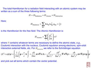
![The total Hamiltonian for a radiation field interacting with an atomic system may be
written as a sum of the three following terms:
Here:
2017
MRT
is the Hamiltonian for the free field. The Atomic Hamiltonian is:
where V contains whatever terms are necessary to define the atomic state, e.g.,
Coulomb interaction with the nucleus, Coulomb repulsion among electrons, spin-orbit
interaction external fields, etc. For HInteraction we refer to the Schrödinger equation
and pick out all terms which contain the vector potential.
nInteractioAtomicRadiation HHHH ++=
∑∑ +=
k
k kk
r
rr aahH ]½)()([ω †
Radiation
V
m
p
H
i
i
+
= ∑ 2
2
Atomic
ψϕϕψϕ
•−•−−•+
+=+′ pAAp ××××∇∇∇∇ΣΣΣΣ∇∇∇∇∇∇∇∇××××∇∇∇∇ΣΣΣΣ 2222
2
23
42
48822
1
)(
cm
e
cm
e
cm
p
mc
e
c
e
m
eE
hhh
164](https://image.slidesharecdn.com/linked-inslides-hydrogen-130507131157-phpapp01/85/Part-V-The-Hydrogen-Atom-164-320.jpg)

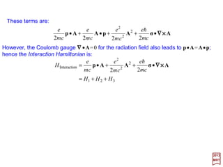
![The total Hamiltonian H=HRadiation +HAtomic +HInteraction may now be written as:
where:
∑∑∑∑ •−+•−
•=•=
k
rk
kk
rk
k
kpkekpke
r
i
rr
r
i
rr a
Vm
e
Ha
Vm
e
H e)(])(ˆ[
ω
2π
e)(])(ˆ[
ω
2π †)(
1
)(
1
hh
and
)(
1
)(
1
†
1 ]e)(e)(][)(ˆ[
ω
2π
+−
•−•
+=
+•= ∑∑
HH
aa
Vm
e
H
r
i
r
i
rr
k
rkrk
k
kkpke
h
With the use of the vector potential obtain A(r)=ΣkΣr êr (k){Ar (k)exp[i(k•r−ωkt)]+
Ar
*(k)exp[−i(k•r−ωkt)]} earlier:
in which H0 contains HRadiation and HAtomic and HInteraction is given by the expression derived
above.
We now assume that HInteraction can be regarded as a perturbation on H0 although, as in
previous cases, the justification is not apparent until the calculations have been
completed. We shall concentrate on the term, H1, of the perturbed Hamiltonian:
nInteractio0 HHH +=
Ap•=
cm
e
H1
which is most often the dominant term in electromagnetic interactions.
2017
MRT
166](https://image.slidesharecdn.com/linked-inslides-hydrogen-130507131157-phpapp01/85/Part-V-The-Hydrogen-Atom-166-320.jpg)
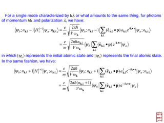
![For a single mode characterized by (k,r) or what amounts to the same thing, for
photons of momentum hk and polarization r, we have:
2017
MRT
in which |ψa〉 represents the initial atomic state and |ψb〉 represents the final atomic
state. In the same fashion, we have:
a
r
i
rb
r
ra
r
i
rrrbrarb
V
n
m
e
nan
Vm
e
nHn
ψψ
ψψψψ
∑∑
∑∑
•
•−
•=
•−=−
k
rk
k
k
rk
k
pke
k
kkpkekkk
e])(ˆ[
ω
)(2π
)(;e)(])(ˆ[1)(;
ω
2π
)(;1)(; )(
1
h
h
a
r
i
rb
r
ra
r
i
rrrbrarb
V
n
m
e
nan
Vm
e
nHn
ψψ
ψψψψ
∑∑
∑∑
•−
•−+
•
+
=
•+=+
k
rk
k
k
rk
k
pke
k
kkpkekkk
e])(ˆ[
ω
]1)([2π
)(;e)(])(ˆ[1)(;
ω
2π
)(;1)(; †)(
1
h
h
167](https://image.slidesharecdn.com/linked-inslides-hydrogen-130507131157-phpapp01/85/Part-V-The-Hydrogen-Atom-167-320.jpg)
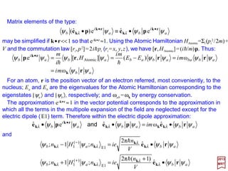
![Matrix elements of the type:
maybesimplifiedif k•r<<1so that eik•r ≈1. Using the Atomic Hamiltonian HAtomic=Σi(pi
2/2m)
+V and the commutation law [ri,p2]=2ihpi (ri =x, y,z), we have [r,HAtomic] =(ih/m)p. Thus:
2017
MRT
For an atom, r is the position vector of an electron referred, most conveniently, to the
nucleus; Ea and Eb are the eigenvalues for the Atomic Hamiltonian corresponding to the
eigenstates |ψa〉 and |ψb〉, respectively; and ωab =ωk by energy conservation.
The approximation eik•r ≈1 in the vector potential corresponds to the approximation in
which all the terms in the multipole expansion of the field are neglected except for the
electric dipole (E1) term. Therefore within the electric dipole approximation:
and:
a
i
bra
i
rb ψψψψ rkrk
pkepke ••
•≡• e)(ˆe])(ˆ[
ab
abbaabababa
i
b
mi
miEE
mi
H
i
m
ψψ
ψψψψψψψψ
r
rrrp
k
rk
ω
ω)(],[e Atomic
=
=−==•
hh
abrabra
i
br im ψψψψψψ rkepkepke k
rk
•=•• •
)(ˆω)(ˆe)(ˆ and
abr
r
rarb
abr
r
rarb
V
n
ienHn
V
n
ienHn
ψψψψ
ψψψψ
rke
k
kk
rke
k
kk
•
+
=+
•=−
+
−
)(ˆ
]1)([2π
)(;1)(;
)(ˆ
)(2π
)(;1)(;
E1
)(
1
E1
)(
1
h
h
168](https://image.slidesharecdn.com/linked-inslides-hydrogen-130507131157-phpapp01/85/Part-V-The-Hydrogen-Atom-168-320.jpg)
](ˆˆ[
ω
)](ˆˆ[
2
ω
)](ˆ[
)()](ˆ[)]()(ˆ[)]()(ˆ[)()(ˆ
2
1
2
1
2
1
2
1
A
rrBrr
rrrr
e
m
i
e
m
i
c
i
i
iiiO
××××××××××××××××
××××
µ
h
SA
2
1
2
1
)()(ˆ)()(ˆ)(ˆ)]()(ˆ[
OO
iiii rrrr
+≡
•+•+•−•=••≡•• kprrpkekprrpkekrpkerkpke
LL
k
k
µkBµkekkk •=•−== −−
)()](ˆˆ)[(
ω2π
)(
ω
2π )(
A
)(
1 rrrr a
V
iOa
Vm
e
H ××××
hh
µB is the Bohr magneton and µµµµL (=µBL) the magnetic moment operator associated with
the orbital angular momentum L. The vector k××××êr (k) lies in the direction of the magnetic
field as is evidentfrom B(r)=iΣkΣr√(2πhωk/V )[k××××êr (k)][ar (k)exp(ik•r)−ar
†(k)exp(−ik•r)].
The connection with the magnetic field can be made more explicit by writing the
complete interaction asociated with OA. From our previous definition for H1
(−), we get:
ˆ
ˆ
where Br
(−)(k)is the term containingar(k) inB(r)=iΣkΣr√(...)[k××××êr(k)][ar(k)exp(ik•r)−...].ˆ
169](https://image.slidesharecdn.com/linked-inslides-hydrogen-130507131157-phpapp01/85/Part-V-The-Hydrogen-Atom-169-320.jpg)
(
)ˆˆˆ()ˆˆ()(
2
1
2
1
M1
)2(
zx
zyxzxx
pxpzki
pppxzki
−=
++•−=•=
kjieepA l
)()( 2
1
M1
)2(
zyy pypzki −=•=
pA l
which corresponds to the polarization vector êr(k) pointing in the direction of the y-axis
since then k××××êr(k) is in the direction of the negative x-axis giving:ˆ
)()()()](ˆˆ[ 2
1
2
1
2
1
A zyxr pypzkikikiO −=×−=ו= prprkek ××××
170](https://image.slidesharecdn.com/linked-inslides-hydrogen-130507131157-phpapp01/85/Part-V-The-Hydrogen-Atom-170-320.jpg)
![2017
MRT
in which µµµµJ is the total magnetic moment operator associated with both orbital and
spin angular momenta.
There is really no need to limit the magnetic moment operators to those which are
associated with the orbital angular momentum. We may as well include the spin which
will now take into amount the term proportional to ΣΣΣΣ•∇∇∇∇××××A in HInteraction. This amounts to
adding 2S to L in OA =−i(mωk/e)[k××××êr(k)]•µµµµL. Hence the matrix elementsformagnetic
(M1) transitions may now be written as:
ˆ
aBbr
r
abr
r
rarrbrarb
V
n
i
V
n
i
nnnHn
ψµψ
ψψ
ψψψψ
)2()](ˆˆ[
)(ω2π
)](ˆˆ[
)(2π
)(;)(1)(;)(;1)(; )(
M1
)(
1
SLkek
k
µkek
k
kkBµkkk
k
J
J
+•=
•−=
•−−=− −−
××××
××××
h
h
aBbr
r
abr
r
rarrbrarb
V
n
i
V
n
i
nnnHn
ψµψ
ψψ
ψψψψ
)2()](ˆˆ[
]1)([ω2π
)](ˆˆ[
]1)([2π
)(;)(1)(;)(;1)(; )(
M1
)(
1
SLkek
k
µkek
k
kkBµkkk
k
J
J
+•
+
−=
•
+
=
•−+=+ ++
××××
××××
h
h
and:
171](https://image.slidesharecdn.com/linked-inslides-hydrogen-130507131157-phpapp01/85/Part-V-The-Hydrogen-Atom-171-320.jpg)
![For the symmetric operator OS, we have:
The replacement of p according to [r,HAtomic] = (ih/m)p gives:
2017
MRT
and:
which is identified as an operator as being the electric quadrupole (E2).
krrkekrrke ••−=••−−= abr
ba
abrabab
m
EE
m
O ψψψψψψ )(ˆ
2
ω
)(ˆ)(
2
S
h
kprrpke •+•= )()(ˆ2
1
S riO
krrkekrrrrke ••=•+•−= ]),[)(ˆ
2
]),[],([)(ˆ
2
AtomicAtomicAtomicS H
m
HH
m
O rr
hh
jirQ δ2
2
1−= rr
which is an irreducible tensor of rank 2. We now have:
)(2
1
S zx pxpzkiO +=
kke
kkekke
k
k
ˆ)(ˆ
2
ω
)(ˆ
2
ω
)(ˆ
2
ω
2
S
••−=
••−=••−=
abr
abrabr
ba
ab
Q
c
m
Q
m
Q
m
O
ψψ
ψψψψψψ
The operator rr is a symmetric Cartesian tensor of rank 2. It is observed that
êr(k)•〈ψb|r2δij |ψa〉•k=〈ψb|r2δij |ψa〉êr(k)•k=0 as a consequence of the transversality
condition (i.e., ∇∇∇∇••••A=0 ⇒ êr (k)•k=0). Therefore rr may be replaced by:
ˆ ˆ
ˆ
The multipole character of OS =(m/2h)êr(k)•[rr,HAtomic] may be investigated:
172](https://image.slidesharecdn.com/linked-inslides-hydrogen-130507131157-phpapp01/85/Part-V-The-Hydrogen-Atom-172-320.jpg)
![The matrix elements for electric quadrupole (E2) transitions may now be written as:
2017
MRT
kke
k
kk k ˆ)(ˆ
)(ω2π
2
)(;1)(;
3
E2
)(
1 ••−=− −
abr
r
rarb Q
V
n
c
e
nHn ψψψψ
h
and:
kke
k
kk k ˆ)(ˆ
]1)([ω2π
2
)(;1)(;
3
E2
)(
1 ••
+
=+ +
abr
r
rarb Q
V
n
c
e
nHn ψψψψ
h
The discussion up to this point involved the interaction of a radiation field with a single
electron. We shall now summarize the important expressions and put them in the form
applicable to a multi-electron system. However, we shall continue to use a single mode
characterized by (k,r). For a system containing N electrons let:
where rj is the position vector of the j-th electron. For an atom the natural reference is
the nucleus; more generally, as in molecules, rj is referred to the center of gravity of the
positive charge.
∑=
=
N
j
j
1
rR
173](https://image.slidesharecdn.com/linked-inslides-hydrogen-130507131157-phpapp01/85/Part-V-The-Hydrogen-Atom-173-320.jpg)
![The interaction matrix elements are then the following:
2017
MRT
kke
k
kk
kke
k
kk
k
k
ˆ)(ˆ
]1)([ω2π
2
)(;1)(;
ˆ)(ˆ
)(ω2π
2
)(;1)(;
E2
3
E2
)(
1
3
E2
)(
1
••
+
=+
••−=−
∑
∑
+
−
a
j
jbr
r
rarb
a
j
jbr
r
rarb
Q
V
n
c
e
nHn
Q
V
n
c
e
nHn
ψψψψ
ψψψψ
h
h
:)(QuadrupoleElectric
a
j
j
br
r
rarb
a
j
j
br
r
rarb
V
n
inHn
V
n
inHn
ψψψψ
ψψψψ
∑
∑
•
+
=+
•−=−
+
−
J
J
µkek
k
kk
µkek
k
kk
)](ˆˆ[
]1)([2π
)(;1)(;
)](ˆˆ[
)(2π
)(;1)(;
M1
M1
)(
1
M1
)(
1
××××
××××
h
h
:)(DipoleMagnetic
abr
r
rarb
abr
r
rarb
V
n
ienHn
V
n
ienHn
ψψψψ
ψψψψ
Rke
k
kk
Rke
k
kk
•
+
=+
•=−
+
−
)(ˆ
]1)([2π
)(;1)(;
)(ˆ
)(2π
)(;1)(;
E1
E1
)(
1
E1
)(
1
h
h
:)(DipoleElectric
174](https://image.slidesharecdn.com/linked-inslides-hydrogen-130507131157-phpapp01/85/Part-V-The-Hydrogen-Atom-174-320.jpg)
![In the description of absoption and emission processes in atoms it is often permissible to
replace the totality of atomic states by just two discrete states between which the
transition occurs (see Figure – zero point energy has been omitted).
2017
MRT
Such a simplification is possible if the energy separation between two states of an
atom correspond to the photon energy hω whereas all other levels are spaced so that
there are no energy differences close to hω. Assuming this to be the case we consider
an atom in the state |ψa〉 interacting with a radiation field described by |nr (k)〉. The initial
state of the entire system, i.e., atom plus field, is |ψA〉=|ψa;nr (k)〉. If absorption takes
place, the atom makes a transition to the state |ψb〉 and there is one photon fewer in the
field. Hence the final state of the system is |ψB〉=|ψb;nr (k)−1〉.* Thus:
Transition Probabilities
|ψb 〉
ABSORPTION EMISSION
|ψa 〉
|ψb 〉
|ψa 〉
|ψa 〉
|ψb 〉
|ψa 〉
|ψb 〉
|ψA〉 = |ψa ; n〉
EA = Ea + nhω
|ψB〉 = |ψb ; n – 1〉
EB = Eb + (n – 1)hω
|ψB〉 = |ψb ; n + 1〉
EB = Eb + (n + 1)hω
|ψA〉 = |ψa ; n〉
EA = Ea + nhω
* In this notation reference to other atomic states or other photons is suppressed since they are not involved in the physical
process.
( )
( )
)ωω(ω
ω]½)([1)(;
ω]½)([)(;
kk
k
k
kk
kk
−=−−=−
−+=−=
++==
baabAB
rbBrbB
raAraA
EEEE
nEEn
nEEn
hh
h
h
ψψ
ψψ
in which Ea and Eb are the energies of the initial and final atomic states, respectively,and:
abba EE −=ωh
175](https://image.slidesharecdn.com/linked-inslides-hydrogen-130507131157-phpapp01/85/Part-V-The-Hydrogen-Atom-175-320.jpg)
![If it is stipulated that the Hamiltonian is independent of time, as will henceforth be
assumed, a formal solution to the Schrödinger equation ih∂tΨΨΨΨ(r,t)=HΨΨΨΨ(r,t) is:
in which the exponential operator is interpreted as:
2017
MRT
Comparing ψ(t)=U(t,to)ψ(to) with ΨΨΨΨ(r,t)=exp[iHo(t−to)/h]ΨΨΨΨ(r,to), it is seen that an
explicit form for the evolution operator is:
Another formulation for the evolution operator is obtained by converting ih∂tU(t,to)=
HU(t,to) and condition U(to,to)=1 into the integral equation:
)(
o
o
e),(
ttH
i
ttU
−−
= h
),(e),( o
)( o
tt
ttH
i
rr ΨΨΨΨΨΨΨΨ
−−
= h
∫ ′′−=
t
t
tdttUH
i
ttU
o
),(1),( oo
h
K
hh
h +−
+−+=
−−
2
o
2
2
o
)(
)(
1
!2
1
)(
1
1e
o
ttH
i
ttH
i
ttH
i
177](https://image.slidesharecdn.com/linked-inslides-hydrogen-130507131157-phpapp01/85/Part-V-The-Hydrogen-Atom-177-320.jpg)
![We now consider the formal interaction representation which is particularly appropriate
for certain formulation of time-dependent perturbation theory.
2017
MRT
and an operator AI(t) in the same representation is given by:
The time derivative of ψI(t) is:
This is an equation of motion for the wave function in the interaction representation
while the other equation of motion is for the operators AI(t):
)(e)(
o
I tt
tH
i
ψψ h=
tH
i
tH
i
tAtA
oo
e)(e)(I
hh
−
=
t
t
tH
i
t
t tH
i
tH
i
∂
∂
+=
∂
∂ )(
e)(e
)( oo
o
I ψ
ψ
ψ hh
h
and upon substituting ih∂ψ/∂t=Hψ =(Ho +V)ψ, we find:
)()()(eee)(e
)(
II
I oooo
ttVtVtV
t
t
i
tH
i
tH
i
tH
i
tH
i
ψψψ
ψ
===
∂
∂ −
hhhhh
]),([
)(
oI
I
HtA
t
tA
i =
∂
∂
h
Let the time-independent Hamiltonian H in the Schrödinger representation be written
as the sum of two parts Ho +V and a wave function ψI(t) in the interaction representation
is defined by:
182](https://image.slidesharecdn.com/linked-inslides-hydrogen-130507131157-phpapp01/85/Part-V-The-Hydrogen-Atom-182-320.jpg)
![We now define an operator UI(t,to) by:
with:
Upon combining ψ(t)=U(t,to)ψ(to) with ψI(t)=exp(iHot/h)ψ(t) one finds:
2017
MRT
from which it is concluded that:
with the second equality based on U(t,to)=exp[−iH(t−to)/h].
The unitarity property of U(t,to) confers unitarity of UI(t,to) so that:
)(),()( oIoII tttUt ψψ =
ooooooo
eeee),(e),(
)(
ooI
tH
i
ttH
i
tH
i
tH
i
tH
i
ttUttU hhhhh
−−−−
==
1),( ooI =ttU
)(e),(e)(),(e)(e)( oIoooI
ooooo
tttUtttUtt
tH
i
tH
i
tH
i
tH
i
ψψψψ hhhh
−
===
),(),( o
1
Io
†
I ttUttU −
=
We may now also find the differential equation obeyed by UI(t,to) by substituting ψI(t)=
UI(t,to)ψI(to) into ih∂ψI(t)/∂t=VI(t)ψI(t). Since ψI(to) is constant:
),()(
),(
oII
oI
ttUtV
t
ttU
i =
∂
∂
h
183](https://image.slidesharecdn.com/linked-inslides-hydrogen-130507131157-phpapp01/85/Part-V-The-Hydrogen-Atom-183-320.jpg)
![We shall now let:
and if we specialize to the case of a transition between the stationary states ϕa and ϕb,
the transition probability is:
The equality between the two forms in the above for wba arises as a result of UI(t,to)=
exp(iHot/h)U(t,to)exp(−iHoto/h) which merely introduces a phase factor into the matrix
elements when U(t,to) is replaced by UI(t,to). Since the probability is determined by the
absolute square of the matrix elements, such phase factors are of no consequence. We
shall use the form |〈ϕb|UI(t,to)|ϕa〉|2 to evaluate the probability per unit time:
2017
MRT
Since the time dependence of 〈ϕb|UI(t,to)|ϕa〉 is contained entirely in the operator UI(t,to)
which satisfies ih∂UI(t,to)/∂t=VI(t)UI(t,to), we have:
bbbaaa EHEHVHH ϕϕϕϕ ==+= ooo and,
2
oI
2
o ),(),( ababba ttUttUW ϕϕϕϕ ==
]),(),([),(
*
oIoI
2
oI abababba ttUttU
td
d
ttU
td
d
W ϕϕϕϕϕϕ ==
]),(),()(Im[
2
]),(),()([
]),()(),(),(),()([
*
oIoII
oIoII
*
oIIoI
*
oIoII
abab
abab
ababababba
ttUttUtV
ttUttUtV
i
ttUtVttUttUttUtV
i
W
ϕϕϕϕ
ϕϕϕϕ
ϕϕϕϕϕϕϕϕ
h
h
h
=
−−=
−=
conjugatecomplex
184](https://image.slidesharecdn.com/linked-inslides-hydrogen-130507131157-phpapp01/85/Part-V-The-Hydrogen-Atom-184-320.jpg)
![We shall now insert(i.e.,using AI(t)=exp(iHot/h)A(t)exp(−iHot/h) and UI(t,to)=exp(iHot/h)
×exp[−iH(t–to)/h]exp(−iHoto/h)) VI(t)=exp(iHot/h)Vexp(−iHot/h) andUI(t,to)=UI(t,0)UI(0,to)=
exp(iHot/h)exp(−iHt/h)UI(0,to) into Wba =(2/h)Im[〈ϕb|VI(t)UI(t,to)|ϕa〉〈ϕb|UI(t,to)|ϕa〉*] to
obtain:
Up to this point to was arbitrary; it will now be assumed that to →−∞. This will allow us
to apply the perturbation V in adiabatically by which it is meant that V is multiplied by the
convergence factor exp(−ε|t|/h) (ε >0). This is a convenient mathematical device and has
the effect of causing the perturbation to vanish at very early and very late times but to
remain unaffected at t=0. Therefore, with ψa=UI(0,−∞)ϕa an eigenfunction of H with
eigenvalue Ea we get:
2017
MRT
which is the reaction matrix.
with:
abba VR ψϕ=
=
−−
*
oIoI ),0(ee),0(eeIm
2 oo
a
tH
i
tH
i
ba
tH
i
tH
i
bba tUtUVW ϕϕϕϕ hhhh
h
]Im[
2
]Im[
2
eeeeIm
2
*
**
abba
abab
tE
i
ab
tE
i
tE
i
ab
tE
i
ba
R
VVW
aaaa
ψϕ
ψϕψϕψϕψϕ
h
hh
hhhh
=
=
=
−−
185](https://image.slidesharecdn.com/linked-inslides-hydrogen-130507131157-phpapp01/85/Part-V-The-Hydrogen-Atom-185-320.jpg)
![We shall now replace ψa in Wba =(2/h)Im[Rba〈ϕb|ψa〉*] by the Lippmann-Schwinger
equation (stated here without proof):
where we use the notation ψI(−∞)=ϕa and ψI(0)=ψa with the assumption that VI(−∞)=0
and Hoϕa =Eaϕa. By the way, this permits us to identifyUI(0,−∞)=1+limε →0[1/(Ea−H+iε)]V.
We then get:
2017
MRT
so that the final result is the Fermi Golden Rule:
Now:
)(
π2 2
bababa EERW −= δ
h
a
a
aa V
iHE
ψ
ε
ϕψ
ε ++
+=
→ o0
1
lim
++
+==
→
*
o0
** 1
limIm
2
]Im[
2
a
a
bbaabbaabbaba V
iHE
RRRW ψ
ε
ϕϕϕψϕ
εhh
Assuming ϕa ≠ϕb, the first term in the brackets vanishes and:
++
=
++
=
→→ εε
ψϕ
εε iEE
R
iEE
V
RW
ba
ba
ba
ab
baba
2
0
*
0
limIm
2
limIm
2
hh
)(π
)(
lim
)(
1
Im 22022 ba
bababa
EE
EEEEiEE
−=
+−+−
=
++ →
δ
ε
ε
ε
ε
ε ε
and
186](https://image.slidesharecdn.com/linked-inslides-hydrogen-130507131157-phpapp01/85/Part-V-The-Hydrogen-Atom-186-320.jpg)
![Physically it is more meaningful to assume a distribution of modes within a narrow
range of frequencies. For a radiation field in a cubical enclosure, according to dN=
[V/(2π)3]k2dkdΩ, the number of modes per unit energy interval is:
2017
MRT
We shall therefore replace the infinitely sharp density distribution δ(Eb −Ea −hωk) in
WAbsorption by (1/h)dN/dωk above to obtain:
Here α =e2/hc is the fine structure constant and quantities such as ωk and nr(k) must be
understood as averages within the interval.
For emission, the calculation goes through in exactly the same way but with the matrix
elements:
Ω= d
c
V
d
dN 2
33
ω
)π2(ω
1
k
k hh
Ω•= d
c
n
dW abr
r 2
2
3
Absorption )(ˆ
π2
)(ω
ψψ
α
Rke
kk
abr
r
rarb
V
n
ienHn ψψψψ Rke
k
kk •
+
=+ +
)(ˆ
]1)([2π
)(;1)(; E1
)(
1
h
The final result, analogous to that in dWAbsorption above is:
Ω•
+
= d
c
n
dW abr
r 2
2
3
Emission )(ˆ
π2
]1)([ω
ψψ
α
Rke
kk
188](https://image.slidesharecdn.com/linked-inslides-hydrogen-130507131157-phpapp01/85/Part-V-The-Hydrogen-Atom-188-320.jpg)
![If W(b,a) represents the transition probability per unit time from the state |αa;Ja,Ma〉
with degeneracy ga to the state with degeneracy gb where αa and αb represent the
quantum numbers required to complete the specification of the states |ψa 〉 and |ψb〉,
respectively, we shall have, in place of WAbsorption =(4αω3n/3c2)|〈ψb|R|ψa〉|2 and WEmission =
[4αω3(n+1)/3c2)]|〈ψb|R|ψa〉|2, we have:
2017
MRT
In these expressions the probabilities for all possible transitions |αa;Ja,Ma〉→|αb;Jb,Mb〉
have been added, but since the probability of an electron being in any one of the initial
states |αa;Ja,Ma〉 is 1/ga, the sum of the probabilities must be multiplied by the factor.
WInduced and WSpontaneous are correspondingly modified. Note that:
where W(b,a) stands for either WAbsorption(b,a) or WEmission(b,a) and the same for W(a,b).
),(),( abW
g
g
baW
b
a
=
∑∑
∑∑
+
=
=
a b
a b
M M
aaabbb
a
M M
aaabbb
a
MJMJ
c
n
g
abW
MJMJ
c
n
g
abW
2
2
3
Emission
2
2
3
Absorption
,;,;
3
)1(ω41
),(
,;,;
3
ω41
),(
αα
α
αα
α
R
R
191](https://image.slidesharecdn.com/linked-inslides-hydrogen-130507131157-phpapp01/85/Part-V-The-Hydrogen-Atom-191-320.jpg)
![Let us now suppose that the population (atoms per cm3) in |ψa 〉 and |ψb〉 are Na and Nb,
respectively. When the system is in equilibrium, the number of transitions per unit time
|ψa 〉→|ψb〉 will be equal to the number of transitions per unit time |ψb〉→|ψa〉 or:
where a refers to the lower state and b to the upper state (see Figure – where the
radiative transitions between two levels are shown).
2017
MRT
In terms of the Einstein coefficients:
)],(),([),( StimulatedInducedAbsorption baWbaWNabWN ba +=
Planck’s Law
|ψ a〉
|ψ b〉
WSponteneous(a,b) WInduced(a,b) WAbsorption(b,a)
)],()ω(),([)ω(),( baAIbaBNIabBN ba +=
But:
),(
ω
π
),(),(
ω
π
),( 3
32
3
32
baA
g
gc
abBbaA
c
baB
a
b
hh
== and
195](https://image.slidesharecdn.com/linked-inslides-hydrogen-130507131157-phpapp01/85/Part-V-The-Hydrogen-Atom-195-320.jpg)
![Also, the equilibrium population satisfies the Boltzmann distribution*:
where Ei is the separation in energy between the states – in this case |ψa〉 and |ψb〉:
2017
MRT
This is known as Planck’s distribution law, where I(ω)dω is the energy per unit volume
(under conditions of thermodynamic equilibrium) for photons in the interval ω to ω+dω.
Tk
E
b
a
b
a B
i
g
g
N
N
e=
1e
1
π
ω
)ω( ω32
3
−
= TkB
c
I h
h
Note that Planck’s law is independent of degeneracies (i.e., ga or gb).
* In chemistry, physics, and mathematics, the Boltzmann distribution is a certain distribution function (or probability measure) for the
distribution of the states of a system. It underpins the concept of the canonical ensemble, providing its underlying distribution. A
special case of the Boltzmann distribution, used for describing the velocities of particles of a gas, is the Maxwell–Boltzmann (M-B)
distribution. So, the Boltzmann distribution for the fractional number of particles Ni /N occupying a set of states i possessing energy Ei
is Ni /N = [gi exp(−Ei /kB T )]/Z(T) where kB is the Boltzmann constant, T is the temperature, gi is the degeneracy (i.e., the number of
levels having energy Ei), N = ΣiNi is the total number of particles and Z(T) = Σigi exp [−Ei/kB T ] is the partition function which encodes
the statistical properties of a system in thermodynamic equilibrium. Alternatively, for a single system at a well-defined temperature, it
gives the probability that the system is in the specified state. The Boltzmann distribution applies only to particles at a high enough
temperature and low enough density that quantum effects can be ignored, and the particles are obeying M-B statistics. When the
energy is simply the kinetic energy of the particle Ei = ½mv2 then the distribution correctly gives the M-B distribution of gas
molecule speeds, previously predicted by James C. Maxwell (1831-1879) in 1859. [Source: Wikipedia] To study this subject
(e.g., canonical ensembles, partition functions, etc.) in its entirety see Feynman, R., Statistical Mechanics (Perseus Books).
Inserting these relations into NaB(b,a)I(ω)=Nb[B(a,b)I(ω)+A(a,b)], we obtain:
ωh=−⇒ abi EEE
196](https://image.slidesharecdn.com/linked-inslides-hydrogen-130507131157-phpapp01/85/Part-V-The-Hydrogen-Atom-196-320.jpg)
![For photon absorption it is necessary to evaluate the matrix elements:
o
o
eee)(ˆ
π
eee)(ˆ
π
1
)(ˆe
2/3
o
2/3
o
s1Free
arZii
r
arZii
rir
i
f
Va
Z
Va
Z
−••
−•••
•
=
•
=•
rkrq
rkrqrk
qke
pkepke
h
ψψ
Coordinate system used in the
calculations.
qkK −−−−=
Defining:
The relationship among the various vectors is shown in the Figure; it is noted
that:
in spherical coordinates. If the coordinate system is oriented so that the z-axis
is along the direction of K and the polarization vector ê along the x-axis:
we have:
∫∫∫ ′′== •
∞
−−•−••
π
00
2
sineeπ2eeeee ooo
θθ drdrd iarZarZiarZii rKrKrkrq
r
222
o
2
3
o
0
π
0 )(
π4
sine
π4
eeesin
2
sine oo
KaZ
aZ
drKrr
K
Kr
rK
d arZarZiii
+
===′′
∫∫
∞
−−••• rkrqrK
andθθ
θ
ϕθ
cos2)(
cossin)(ˆ
2222
qk
qr
−+==
=•
qkqkK
qke
−−−−
2017
MRT
Thus:
])(ˆ[
)(
)(π8
e 222
o
2
2/3
o
qkerk
•
+
=•
ri
i
f
KaZV
ZZa h
ψψ
z
y
x
ê
θ
k
ϕ q
K
e
z
y
x
r
e−
Ze+
o
e
π
1
2/3
o
arZ
i
a
Z −
=ψ
rq•
= i
f
V
e
1
ψ
1s
200](https://image.slidesharecdn.com/linked-inslides-hydrogen-130507131157-phpapp01/85/Part-V-The-Hydrogen-Atom-200-320.jpg)
![It will be assumed that the photon energy is large compared with the binding energy of
the electron in the atom but small compared to the rest mass of the electron. The first
assumption ensures that the final state is that of a free electron and the second avoids
the necessity of a relativistic treatment. Fortunately both conditions are satisfied when:
The first factor on the right is of the order of the binding energy I and the second factor is
2⋅137/Z; hence E is at least several times larger than I. With the assumption that E=I,
the photons energy becomes comparable to thekineticenergyof the electron hck=mov2/2
from which itfollowsthat k/q=v/2c=Z/qao orqao=Z and Z2 +ao
2K2 =Z2 +ao
2(k2 +q2 −2qkcosθ)
≈q2ao
2(1−β cosθ) (with β =v/c). Therefore the matrix element is:
where k=|k| is the photon wave number, ao the Bohr radius, and Z the atomic number of
the atom. To see the justification of this criterion we first calculate the photon energy
corresponding to kao ≈ Z:
and the complete interaction matrix element is:
22
o
2
2/3
o
)]cos1([
cossin)(π8
)(ˆe
θβ
ϕθ
ψψ
−
=••
aqV
qZZa
ir
i
f
h
pkerk
2017
MRT
Zak ≈o
=== 22
4
o
2
o
2
2 eZ
cemZ
a
Zc
kcE
h
h
h
h
ir
i
f
V
n
m
e
ψψ pkerk
••
)(ˆe
ω
π2
o
h
201](https://image.slidesharecdn.com/linked-inslides-hydrogen-130507131157-phpapp01/85/Part-V-The-Hydrogen-Atom-201-320.jpg)
![Higher Order Electromagnetic Interactions
The process of absorption and emission (e.g., the photoelectric absorption Wn(k,q;θ,ϕ))
described earlier are one-photon processes since in every transition the field either loses
or gains a photon while the atom undergoes a corresponding change of state to keep
the total energy (atom plus field) constant.
In the absence of an external magnetic field the Hamiltonian describing the interaction
of an electron with a radiation field is:
There are other important interactions between an atom and a radiation field which
involve a change of more than one photon. In a general scattering event, for example,
the field loses an incident photon characterized by kr (e.g.,aspart of the sums Σk and Σr
seen earlier) and gains another photon – the scattered one with momentum k′ –
characterized by k′s. With laser sources, numerous multiphoton processes have been
observed although the present discussion will be restricted to several aspects of the
two-photon interaction.
where A is given by A(r)=ΣkΣr√(2πhc2/V ωk)êr(k)[ar(k)exp(ik•r)−ar
†(k)exp(−ik•r)] and
the H3 term is neglected.
321
2
2
2
nInteractio
22
HHH
mc
e
cm
e
cm
e
H
++=
•++•= AσAAp ××××∇∇∇∇
h
2017
MRT
203](https://image.slidesharecdn.com/linked-inslides-hydrogen-130507131157-phpapp01/85/Part-V-The-Hydrogen-Atom-203-320.jpg)
![As we’ve done before, we let:
For H2, we have:
in which Hkr
(+)Hk′s
(+) refers to the term containing a†
kr a†
k′s; Hkr
(−)Hk′s
(−) to the term with
ar (k)as(k′), etc.
where:
2017
MRT
{
}
)()()()()()()()(
)(†)(†
)()(††
22
††
22
2
e)()(e)()(
e)()(e)()(
ωω
)(ˆ)(ˆπ
]e)(e)(][e)(e)()][(ˆ)(ˆ[
ωω
1π
+
′
−−
′
+−
′
−+
′
+
•′−•′−−
•′+•′+−
′
•′−•′•−•
′
+++=
′+′+
′+′
′•
=
′+′+′•=
∑∑
∑∑
srsrsrsr
i
sr
i
sr
r
i
sr
i
sr
sr
r
i
s
i
s
i
r
i
rsr
HHHHHHHH
aaaa
aaaa
mV
e
aaaa
mV
e
H
kkkkkkkk
rkkrkk
k
rkkrkk
kk
k
rkrkrkrk
kk
kkkk
kkkk
keke
kkkkkeke
h
h
∑∑∑∑ •−+•−
•=•=
k
rk
kk
rk
k
kpkekpke
r
i
rr
r
i
rr a
Vm
e
Ha
Vm
e
H e)(])(ˆ[
ω
2π
e)(])(ˆ[
ω
2π †)(
1
)(
1
hh
&
)(
1
)(
1
†
1 ]e)(e)(][)(ˆ[
ω
2π
+−
•−•
+=
+•= ∑∑
HH
aa
Vm
e
H
r
i
r
i
rr
k
rkrk
k
kkpke
h
204](https://image.slidesharecdn.com/linked-inslides-hydrogen-130507131157-phpapp01/85/Part-V-The-Hydrogen-Atom-204-320.jpg)
![Matrix elements of ar (k) and ar
†(k) may be obtained from ar (k)|nr (k)〉=√ nr (k)|nr (k)−1〉
and ar
†(k)|nr (k)〉=√[nr (k)+1]|nr (k)+1〉:
which leads directly to:
Since the photon modes are independent we also have:
The only non-vanishing matrix elements of ar
†(k) and ar (k) are those which involve a
change of one photon. For all bilinear combinations of ar
†(k) and ar (k) the change in the
number of photons must be zero or two.
)()()(1)(1)()()(1)( †
kkkkkkkk rrrrrrrr nnannnan =−+=+ and
)()()(),()()(1)(,1)(
]1)()[()(),()()(1)(,1)(
)(]1)([)(),()()(1)(,1)(
]1)(][1)([)(),()()(1)(,1)(
†
†
††
kkkkkkkk
kkkkkkkk
kkkkkkkk
kkkkkkkk
′=′′−′−
+′=′′+′−
′+=′′−′+
+′+=′′+′+
srsrsrsr
srsrsrsr
srsrsrsr
srsrsrsr
nnnnaann
nnnnaann
nnnnaann
nnnnaann
0)](),([)](),([)](),([ †††
=′=′=′ kkkkkk srsrsr aaaaaa
2017
MRT
205](https://image.slidesharecdn.com/linked-inslides-hydrogen-130507131157-phpapp01/85/Part-V-The-Hydrogen-Atom-205-320.jpg)
![We consider a two-level system (see Figure).
)(),(;I kk ′= sri nnψ
Also scattering has occurred, ns (k′) is increased by one photon and nr (k) is decreased
by one photon so that the total system is now in the state |F 〉:
with energy (N.B., not including the zero point energy):
ssrri nnEE kk kk ′′++= ω)(ω)(I hh
with energy:
2017
MRT
1)(,1)(;F +′−= kk srf nnψ
ssrrf nnEE kk kk ′+′+−+= ω]1)([ω]1)([F hh
The energy Ei relative to Ef is arbitrary and the scattered photon may have more of
less energy compared with the incident photon. This represents the general case of
Raman scattering and includes elastic scattering as a special case.
Initially the atom is in the state |ψi 〉 and two photon modes with occupation numbers
nr (k) and ns (k′) (i.e., simultaneously observable – through momentums k and k′ photon
eigenvalues of the occupation numbers) are present. The total system is in the state |I 〉:
|ψf〉
SCATTERING
|ψi〉
|ψf〉
|ψi〉
| I 〉 = |ψi ; nr(k),ns(k′)〉 | F 〉 = |ψf ; nr(k)−1,ns(k′) +1〉
206](https://image.slidesharecdn.com/linked-inslides-hydrogen-130507131157-phpapp01/85/Part-V-The-Hydrogen-Atom-206-320.jpg)
![From 〈nr (k)+1,ns (k′)+1|ar
†(k)as
†(k′)|nr (k),ns (k′) 〉=√{[nr (k)+1][ns (k′)+1]},
〈nr (k)+1,ns (k′)−1|ar
†(k)as
†(k′)|nr (k),ns (k′)〉=√{[nr (k)+ 1]ns (k′)}, and also
〈nr (k)−1,ns (k′)+1|ar(k)as
†(k′)|nr (k),ns (k′)〉=√{nr (k)[ns (k′)+1]} and finally with
〈nr (k)−1,ns (k′)−1|ar(k)as(k′)|nr (k),ns (k′)〉=√[nr (k)ns (k′)], it follows that:
i
i
fsr
sr
srsr
srsr
nn
mV
e
HHHH
HHHH
ψψ rkk
kk
keke
kk
kkkk
kkkk
•′−
′
+−−+
−−++
′•
+′
=′=′
=′=′
)(
2
)()()()(
)()()()(
e)](ˆ)(ˆ[
ωω
]1)()[(π
I)()(FI)()(F
0I)()(FI)()(F
h
The scattering process is regarded as a two-photon process in the sense that an inci-
dent photon of specified energy, polarization, and propagation direction symbolized by
the indices kr (i.e., a discrete sum for each index) is scattered so that the emerging pho-
ton may have a different energy, polarization, and direction of propagation symbolized by
the indices k′s. Hence, a kr photon has been lost and a k′s photon has been gained!
Therefore:
2017
MRT
i
i
fsr
sr nn
mV
e
H ψψ rkk
kk
keke
kk •′−
′
′•
+′
= )(
2
2 e)](ˆ)(ˆ[
ωω
]1)()[(2π
IF
h
Matrix elements of H1 will be of type ar(k)|nr(k)〉=√nr(k)|nr(k)−1〉 and ar
†(k)|nr(k)〉=
√[nr(k)+1]|nr(k)+1〉 in which where is a chance of one photon. Therefore H1 cannot
contribute to scattering in the first order of perturbation theory but may contribute to
higher order. The matrix elements of H2 are non-vanishing when there is a change
of two photons; first order contributions from H2 are therefore expected.
207](https://image.slidesharecdn.com/linked-inslides-hydrogen-130507131157-phpapp01/85/Part-V-The-Hydrogen-Atom-207-320.jpg)
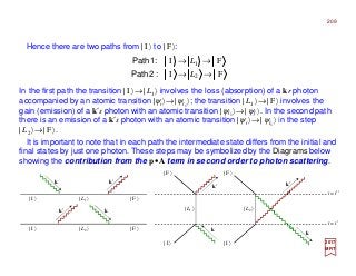
![We saw earlier that H1
(−) was associated with the absorption of a single photon and
H1
(+) with the emission of a single photon. Therefore the matrix elements in the two paths
are the following:
2017
MRT
ir
i
lls
i
f
sr
srisrl
srlsrf
nn
Vm
e
nnHnn
nnHnnHLLH
L
ψψψψ
ψψ
ψψ
])(ˆ[e])(ˆ[e
ωω
]1)()[(2π
)(),(;)(,1)(;
)(,1)(;1)(,1)(;IF
FI
11
1
1
2
2
)(
1
)(
1
)(
111
)(
1
1
pkepke
kk
kkkk
kkkk
rkrk
kk
••′
+′
=
′′−×
′−+′−=
→→
••′−
′
+
+−+
h
For
is
i
llr
i
f
sr
srisrl
srlsrf
nn
Vm
e
nnHnn
nnHnnHLLH
L
ψψψψ
ψψ
ψψ
])(ˆ[e])(ˆ[e
ωω
]1)()[(2π
)(),(;1)(),(;
1)(),(;1)(,1)(;IF
FI
22
2
2
2
2
)(
1
)(
1
)(
122
)(
1
2
pkepke
kk
kkkk
kkkk
rkrk
kk
•′•
+′
=
′+′×
+′+′−=
→→
•′−•
′
+
−+−
h
For
210](https://image.slidesharecdn.com/linked-inslides-hydrogen-130507131157-phpapp01/85/Part-V-The-Hydrogen-Atom-210-320.jpg)
![Both paths contribute to the second-order term in 〈ψk| R|ψm〉=〈ψk |V |ψm〉
+Σl[〈ψk|V |ψl〉〈ψl|V |ψm〉/(Em−El)]. On setting:
the second-order term becomes:
kk ′−−=−+−=− ωω 2211 II hh liLliL EEEEEEEE and
in which the general summation index l indicates the sum over all intermediate states
accessible to one-photon transitions.
2017
MRT
−−
•′•
+
+−
••′+′
′
•′−•
••′−
′
∑
k
rkrk
k
rkrk
kk
pkepke
pkepkekk
ω
])(ˆ[e])(ˆ[e
ω
])(ˆ[e])(ˆ[e
ωω
]1)()[(2π
2
22
1
11
2
2
h
h
h
li
is
i
llr
i
f
l li
ir
i
lls
i
fsr
EE
EE
nn
Vm
e
ψψψψ
ψψψψ
211](https://image.slidesharecdn.com/linked-inslides-hydrogen-130507131157-phpapp01/85/Part-V-The-Hydrogen-Atom-211-320.jpg)
(ˆ[
ωω
]1)()[(2π
)(),(;1)(,1)(;
2
nInteractio
hh
h
li
isllrf
l li
irllsf
ifsr
sr
srisrf
EEEEm
nn
mV
e
nnHnn
ψψψψψψψψ
δψψ
−−
•′•
+
+−
••′+′
′
•′−•
••′−
′
∑
k
rkrk
k
rkrk
kk
pkepke
pkepkekk
ω
])(ˆ[e])(ˆ[e
ω
])(ˆ[e])(ˆ[e
ωω
]1)()[(2π
2
22
1
11
2
2
h
h
h
li
is
i
llr
i
f
l li
ir
i
lls
i
fsr
EE
EE
nn
Vm
e
ψψψψ
ψψψψ
i
i
fsr
sr nn
mV
e
H ψψ rkk
kk
keke
kk •′−
′
′•
+′
= )(
2
2 e)](ˆ)(ˆ[
ωω
]1)()[(2π
IF
h
212](https://image.slidesharecdn.com/linked-inslides-hydrogen-130507131157-phpapp01/85/Part-V-The-Hydrogen-Atom-212-320.jpg)
(ˆ[]1)()[(
ω
ω
−−
•′•
+
+−
••′
+
+′•+′Ω
=
′
′
∑ kk
k
k
pkepkepkepke
kekekk
hh li
isllrf
l li
irllsf
ifsrsr
EEEEm
nnd
V
c
mc
e
W
ψψψψψψψψ
δ
The intermediate states |ψl〉 which appear in theKramers-Heisenbergdispersionformu-
la,aswellastheinitial state |ψi〉 and the final state |ψf 〉 arealleigenstates of theatom, i.e.,
solutions of the atomic Schrödinger equation. By virtue of the existence of matrix ele-
ments between |ψi〉 and |ψl〉 and |ψl〉 and |ψf〉, the two states |ψi〉 and |ψf〉 can interact
via two-photon processes. However, the transition |ψi〉→|ψl 〉 and |ψl 〉→| ψf 〉 are not
observable – the states |ψl〉 are sometimes called “virtual” because of this feature.
213](https://image.slidesharecdn.com/linked-inslides-hydrogen-130507131157-phpapp01/85/Part-V-The-Hydrogen-Atom-213-320.jpg)
(ˆ[]1)([
ω
ω
)(
−−
•′•
+
+−
••′
+
+′•+′=
Ω
=
′
=
Ω
′
′
∑ kk
k
k
pkepkepkepke
kekek
k
k
k
hh li
ilslfr
l li
ilrlfs
ifsrs
r
EEEEm
nr
Vcn
dW
r
s
d
d
ψψψψψψψψ
δ
σ
2
cm-secscattered/photonsincidentofnumber
sr-secscattered/photonsofnumber
electrontheofradiusclassical== 2
2
o
mc
e
r
The formula above for the differential cross section contains the factor [ns(k′′′′)+1];
hence the cross section is a sum of two terms one of which is proportional to ns (k′′′′), the
number of scattered photons. This term corresponds to stimulated Raman scattering;
it contributes negligibly at ordinary intensities, but produces important effects at high
intensities.
214](https://image.slidesharecdn.com/linked-inslides-hydrogen-130507131157-phpapp01/85/Part-V-The-Hydrogen-Atom-214-320.jpg)
![2017
MRT
ir
i
f
r
if
rf
ri
V
n
m
e
HHR
n
n
ψψ
ψ
ψ
])(ˆ[e
ω
)(π2
IFIF
1)(;F
)(;I
)(
11
)1(
pke
k
k
k
rk
k
•===
−=
=
•− h
Starting with the Fermi Golden Rule Wkm =(2π/h)|〈ψk|R|ψm〉|2δ(Ek −Em) in which the
general form of the matrix elements is 〈ψk |R|ψm〉≡Rkm = Rkm
(1)+ Rkm
(2) +…and it is possible
to symbolize these expressions by means of diagrams which are helpful in writing the
pertinent matrix elements associated with a particular process:
Single photon emission:
ir
i
f
r
if
rf
ri
V
n
m
e
HHR
n
n
ψψ
ψ
ψ
])(ˆ[e
ω
]1)([π2
IFIF
1)(;F
)(;I
)(
11
)1(
pke
k
k
k
rk
k
•
+
===
−=
=
•−+ h
k
| I 〉 | F 〉
k
| I 〉 | F 〉
Single photon absorption:
215](https://image.slidesharecdn.com/linked-inslides-hydrogen-130507131157-phpapp01/85/Part-V-The-Hydrogen-Atom-215-320.jpg)
![Processes involving two photons (second order processes) are scattering, two-photon
absorption and two-photon emission. Scattering has already been discussed earlier (the
pertinent diagrams were shown 7 slides ago):
2017
MRT
Two-photon absorption:
∑
∑
∑∑
′
•′•
′
••′
′
−−−−
+−
•′•′
=
+−
••′′
=
+≡
−
+
−
=
−′=−′−=
′−=′=
2 2
22
1 1
11
2 21 1
2
1
ω
])(ˆ[e])(ˆ[e
ωω
)()(π2
ω
])(ˆ[e])(ˆ[e
ωω
)()(π2
IFIF
1)(),(;1)(,1)(;F
)(,1)(;)(),(;I
2
2
4
2
2
3
43
I
)(
122
)(
1
I
)(
111
)(
1)2(
2
1
l li
is
i
llr
i
fsr
l li
ir
i
lls
i
fsr
L LL L
if
srlsrf
srlsri
EE
nn
Vm
e
M
EE
nn
Vm
e
M
MM
EE
HLLH
EE
HLLH
R
nnLnn
nnLnn
k
rkrk
kk
k
rkrk
kk
pkepkekk
pkepkekk
kkkk
kkkk
h
h
h
h
ψψψψ
ψψψψ
ψψ
ψψ
| I 〉 | F 〉| L2 〉
k′ k
where
| I 〉 | F 〉| L1 〉
k k′
216](https://image.slidesharecdn.com/linked-inslides-hydrogen-130507131157-phpapp01/85/Part-V-The-Hydrogen-Atom-216-320.jpg)
![Two-photon emission:
2017
MRT
∑
∑
∑∑
′
•′−•−
′
•−•′−
′
++++
−−
•′+′+
=
−−
••′+′+
=
+≡
−
+
−
=
+′=+′+=
′+=′=
2 2
22
1 1
11
2 21 1
2
1
ω
])(ˆ[e])(ˆ[e
ωω
]1)(][1)([π2
ω
])(ˆ[e])(ˆ[e
ωω
]1)(][1)([π2
IFIF
1)(),(;1)(,1)(;F
)(,1)(;)(),(;I
2
2
6
2
2
5
65
I
)(
122
)(
1
I
)(
111
)(
1)2(
2
1
l li
is
i
llr
i
fsr
l li
ir
i
lls
i
fsr
L LL L
if
srlsrf
srlsri
EE
nn
Vm
e
M
EE
nn
Vm
e
M
MM
EE
HLLH
EE
HLLH
R
nnLnn
nnLnn
k
rkrk
kk
k
rkrk
kk
pkepkekk
pkepkekk
kkkk
kkkk
h
h
h
h
ψψψψ
ψψψψ
ψψ
ψψ
| I 〉 | F 〉| L2 〉
k′ k
where
| I 〉 | F 〉| L1 〉
k k′
217](https://image.slidesharecdn.com/linked-inslides-hydrogen-130507131157-phpapp01/85/Part-V-The-Hydrogen-Atom-217-320.jpg)
(ˆ[
ωω
]1)()[(π2
I)()(F2I)()(F2IF
1)(,1)(;F
)(),(;I
h
k′k
| I 〉 | F 〉
218](https://image.slidesharecdn.com/linked-inslides-hydrogen-130507131157-phpapp01/85/Part-V-The-Hydrogen-Atom-218-320.jpg)
(ˆ[
ωω
)()(π2
I)()(FIF
1)(,1)(;F
)(),(;I
h
Two-photon emission:
i
i
fsr
sr
srif
srf
sri
nn
Vm
e
HHHR
nn
nn
ψψ
ψ
ψ
rkk
kk
keke
kk
kk
kk
kk
•′+−
′
++
′•
+′+
=
′==
+′+=
′=
)(
2
)()(
2
)1(
e)](ˆ)(ˆ[
ωω
]1)(][1)([π2
I)()(FIF
1)(,1)(;F
)(),(;I
h
k′k
| I 〉 | F 〉
k′
k
| I 〉 | F 〉
219](https://image.slidesharecdn.com/linked-inslides-hydrogen-130507131157-phpapp01/85/Part-V-The-Hydrogen-Atom-219-320.jpg)

![Epilogue
“Where did we get that [equation] from? Nowhere. It is not possible to derive
it from anything you know. It came out of the mind of Schrödinger!”
Richard Feynman
),(),(ˆ t
t
itH rr ΨΨΨΨΨΨΨΨ
∂
∂
= h
2017
MRT
221](https://image.slidesharecdn.com/linked-inslides-hydrogen-130507131157-phpapp01/85/Part-V-The-Hydrogen-Atom-221-320.jpg)
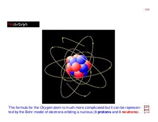
![Ice forms as a Hydrogen bond between water molecules by a polar H bond: δ+-δ−.
H bond
H2O (1s[1 -1s22s2p[2] -1s1])
2017
MRT
223](https://image.slidesharecdn.com/linked-inslides-hydrogen-130507131157-phpapp01/85/Part-V-The-Hydrogen-Atom-223-320.jpg)
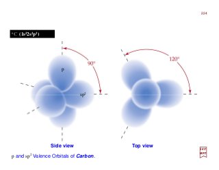
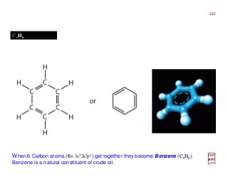
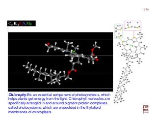
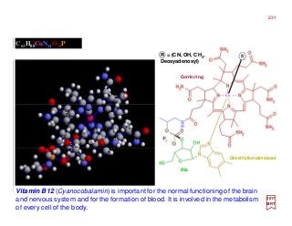
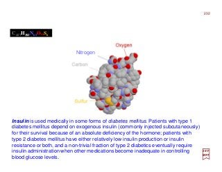
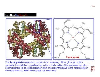
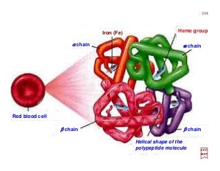

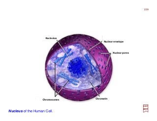

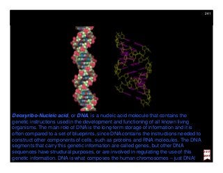
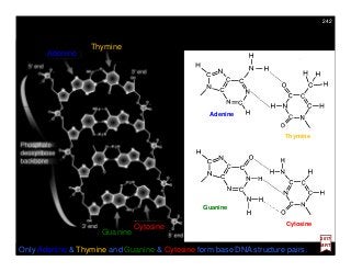
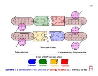
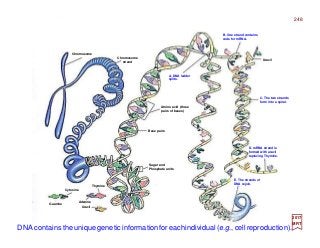
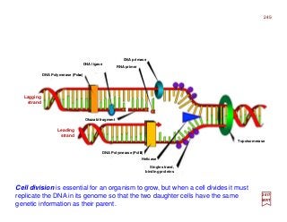
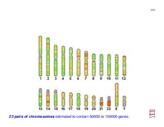
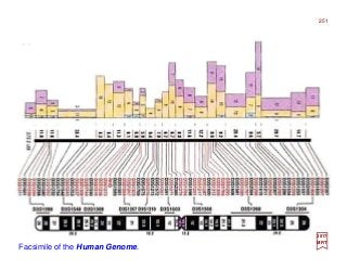


The document summarizes key details about the hydrogen atom and its electron orbital structure based on quantum mechanics. It provides: 1) A direct observation of the electron orbital of a hydrogen atom placed in an electric field, obtained through photoionization microscopy. Interference patterns observed directly reflect the nodal structure of the wavefunction. 2) Calculated and measured probability patterns for the electron in different energy levels of the hydrogen atom are shown. Bright regions correspond to high probability of finding the electron. 3) An overview of solving the radial, angular and azimuthal coordinate functions of the hydrogen atom through series expansion, as exact solutions have not been found. Approximate solutions can be obtained for more complex atoms like he