Downloaded 143 times
![8
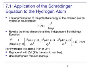
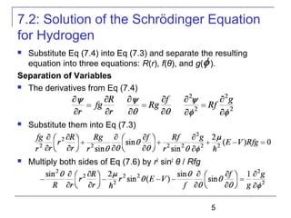
Solution of the Schrödinger Equation
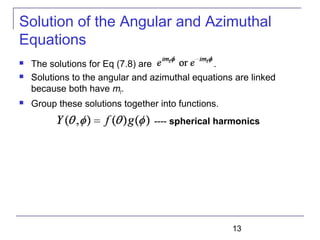
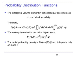
Set each side of Eq (7.9) equal to constant ℓ(ℓ + 1).
Schrödinger equation has been separated into three ordinary
second-order differential equations [Eq (7.8), (7.10), and (7.11)],
each containing only one variable.
----Radial equation
----Angular equation](https://image.slidesharecdn.com/trm-7-161116011803/85/Trm-7-8-320.jpg)
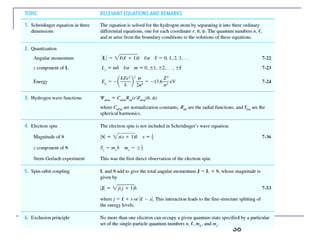

The document summarizes key concepts about the hydrogen atom from quantum mechanics. It begins by introducing the Schrödinger equation and how it can be applied and solved for the hydrogen atom potential. The solution involves separation of variables into radial, angular, and azimuthal components. This leads to the identification of three quantum numbers - principal (n), angular momentum (l), and magnetic (ml) - that characterize the possible energy states. Higher sections discuss properties like orbital shapes, spin, and transition selection rules between energy levels and electron probability distributions.


![บทที่ 1 หน่วยวัดและปริมาณทางฟิสิกส์ [2 2560]](https://cdn.slidesharecdn.com/ss_thumbnails/12-2560-180110052203-thumbnail.jpg?width=640&height=640&fit=bounds)


