Downloaded 48 times

![7
Particles are
electrons
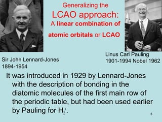
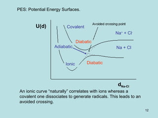
Born-Oppenheimer
approximation
1927
Max Born German
(1882-1970)
Julius Robert Oppenheimer
Berkeley- Los alamos
1904 –1967
HH = [Te +VN-e + Vee] + TN + VN-N
HHee = [Te +VN-e + Vee]
Ψ = ΠΨ(e) ΠΨ(Ν)
e N
VN-e also acts on N; when N is
considered as fixed: VN-e then
becomes an operator acting on e.
Separation of Ψ(e) and Ψ(N)
Should be a
coupling term
}Operator acting on e](https://image.slidesharecdn.com/hartree-focktheory-190113194316/85/Hartree-fock-theory-7-320.jpg)


![31
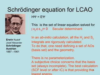
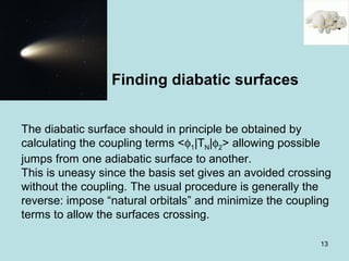
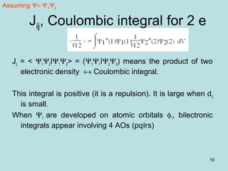
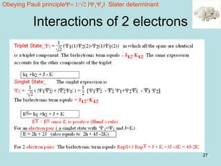
Slater rules
Non zero terms arise from 3 possibilities:
• Dl = DR <DlIOIDR> = Σ [<kikjIOIlilj> - <kikjIOIlilj>]
• Dl differ from DR by one orbital i
<DlIOIDR> = <kiIOIlj>
<DlIOIDR> = Σ [<kikjIOIlilj> - <kikjIOIlilj>]
• Dl differ from DR by two orbitals i and j
<DlIOIDR> = <kikjIOIlilj> - <kikjIOIlilj>
i<j
N
i≠
j
N](https://image.slidesharecdn.com/hartree-focktheory-190113194316/85/Hartree-fock-theory-31-320.jpg)
![33
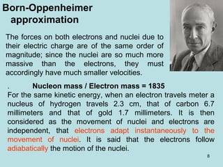
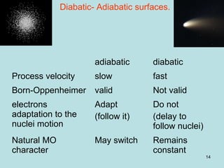
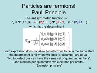
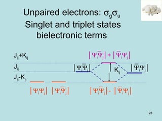
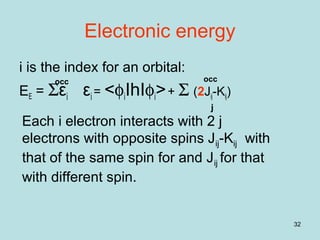
Electronic energy – total energy
The sum of the energies of all the electrons
contains the ij repulsion twice:
EE = Σεi εi = <φiIhIφi>+ Σ (2Jij-Kij)
occocc
i
EE = Σ[hii + Σ repij
occ
ji
occ
= Σ [hii+2 Σ Repij
j
occ occ
] ]
ESCF = <ΨSCFIHIΨSCF> = Σhii + Σ Σ(2Jij-Kij)
j<ii
occ occ
ESCF +ENETOTAL =
ESCF is defined as the energy of ΨSCF applying Slater rules
ESCF = EE - Repij = Σhii + Repij
i
i
occPauli principle
occ
i](https://image.slidesharecdn.com/hartree-focktheory-190113194316/85/Hartree-fock-theory-33-320.jpg)
![34
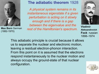
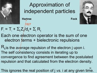
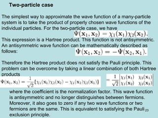
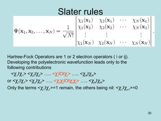
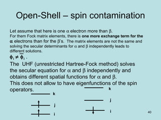
Restricted Hartree-Fock
Closed-shell system: an MO is doubly occupied or
vacant. The spatial functions are independent from the
spin. Assuming k and l with spin α, the expression of
a Fock matrix-element, Fkl, is
Fkl = h + 2J – K and
εi = hii + Σ (2Jij-Kij)
ESCF = 2Σ εi – ΣΣ(2Jij-Kij)
occ occ
J of spin α J of spin β
Fkl = hkl + Σ [(klIjj)-(klIjj)] - Σ (klIjj)
occ
j
occ occ occ
i j<ii
There is no exchange
term for electrons with
different spin (<αΙβ>=0)
Altogether there are 2 J
for one K.](https://image.slidesharecdn.com/hartree-focktheory-190113194316/85/Hartree-fock-theory-34-320.jpg)


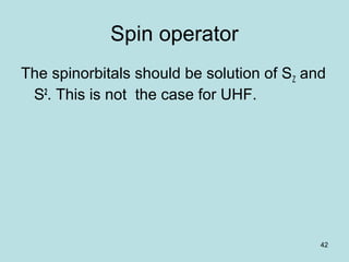
![41
ROHF
The same spatial function is taken whatever the
spin is.
Robert K. Nesbet
This allows eigenfunctions of spin operators.
This allows separating spatial and spin functions.
It is not consistent with variational principle (that
does better without this constraint).
F = h + Σ [( Ijj)-( jI j)] - Σ ( Ijj)-1/2 ( jI j)
2e occ 1e occ
j j](https://image.slidesharecdn.com/hartree-focktheory-190113194316/85/Hartree-fock-theory-41-320.jpg)

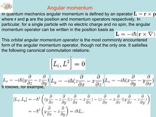
![45
L2
is the norm and Lx, Ly, Lz are the projections.
[Jx, Jy]= i Jz [Jx, J2
]= 0
[Jy, Jz]= i Jx eigenfunctions of J2
are j(j+1)
[Jz, Jx]= i Jy eigenfunctions of Jz are m
J2
Ij,m> = j(j+1) Ij,m> and Jz Ij,m> = m Ij,m>
Relations in Angular momentum
In atomic units, h =1](https://image.slidesharecdn.com/hartree-focktheory-190113194316/85/Hartree-fock-theory-45-320.jpg)
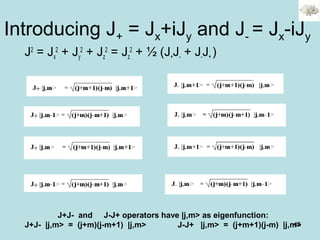

![48
spin
For several electrons: the total spin is the vector sum of the
individual spins.
• For the projection Sz=Ms = Σs ms
• For the norm S2
= S1
2
+S2
2
+2S1S2
S2
=[S1z
2
+S1z+S1-S1+]+[S2z
2
+S2z+S2-S2+]+[(S1+S2- ++S1-S2+)+2S1zS2z]
• For 2 electrons, there are 4 spin functions:
α(1) α(2), β(1) β(2), α(1) β(2) and α(2) β(1) that are
solutions of Sz.
Are they solution of S2
?](https://image.slidesharecdn.com/hartree-focktheory-190113194316/85/Hartree-fock-theory-48-320.jpg)
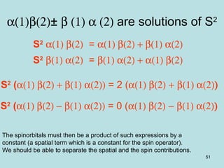
![49
α(1)α(2) is solution of S2
α(1) (Sz
2
+Sz+S-S+) α(2) [1/2]2
+ 1/2 + 0 0.75
α(2) (Sz
2
+Sz+S-S+) α(1) [1/2]2
+ 1/2 + 0 0.75
2Szα(1)Szα(2) 2 ½ ½ 0.5
S-α(1)S+α(2) 0 0
S+α(1)S-α(2) 0 0
total 2
S2
α(1) α(2) = 2 α(1) α(2)](https://image.slidesharecdn.com/hartree-focktheory-190113194316/85/Hartree-fock-theory-49-320.jpg)
![50
α(1)β(2) is not a solution of S2
α(1) (Sz
2
+Sz+S-S+) β(2) [1/2]2
- 1/2 + 1 0.75
β(2) (Sz
2
+Sz+S-S+) α(1) [1/2]2
+ 1/2 + 0 0.75
2Szα(1)Szβ(2) 2 ½ (-½) -.5
S-α(1)S+β(2) β(1) α(2) β(1) α(2)
S+α(1)S-β(2) 0 0
total 2
S2
α(1) β(2) = α(1) β(2) + β(1) α(2)](https://image.slidesharecdn.com/hartree-focktheory-190113194316/85/Hartree-fock-theory-50-320.jpg)
![52
Use of indentation operators
upon vector sums
S2
=Sz
2
+Sz+S-S+
S-S+ |1,1> = 0
S-S+ |1,0> = (1+0+1)(1-0) |1,0> = 2|1,0>
S-S+ |1,-1> = (1-1+1)(1+1) |1,-1> = 2 |1,-1>
Singlet S2
|0,0> = [0+0+0] =0 |0,0>
Triplet S2
|1,1> = [1+1+0] |1,1>
Triplet S2
|1,0> = [0+0+2] |1,0>
Triplet S2
|1,-1> = [1-1+2] |1,-1>](https://image.slidesharecdn.com/hartree-focktheory-190113194316/85/Hartree-fock-theory-52-320.jpg)
![53
S2
as an operator on determinant
S2
(D)= Pαβ(D) + [(nα-nβ)2
+2nα +2nβ ] D
Pαβ is an operator exchanging the spins :α ↔ β
nα and nβ are the # of electrons of each spin
Application:
S2
(IaaI) = IaaI+IaaI = -IaaI+IaaI = 0
S2
(IabI) = IabI+IabI
S2
(IabI-IbaI) = 2 (IabI+IabI)= 2 (IabI-IbaI)
S2
(IabI+IbaI) = IabI+IbaI+IabI+IbaI
= -IbaI-IabI+IabI+IabI = 0](https://image.slidesharecdn.com/hartree-focktheory-190113194316/85/Hartree-fock-theory-53-320.jpg)
![55
A combination of Slater
determinant then may be an
eigenfunction of S2
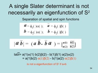
The separation of spatial and spin functions is possible
If the spatial function (a or b) is associated with opposite spins
IabI± IbaI = a(1)b(2) α(1)β(2) - b(1)a(2) α(2)β(1)
are a eigenfunction of S2
± b(1)a(2) α(1)β(2) - a(1)b(2) α(2)β(1)
[a(1)b(2) + b(1)a(2)] (α(1)β(2) - α(2)β(1))IabI+ IbaI =
+
[a(1)b(2) - b(1)a(2)] (α(1)β(2) + α(2)β(1))IabI- IbaI =](https://image.slidesharecdn.com/hartree-focktheory-190113194316/85/Hartree-fock-theory-55-320.jpg)
β(2) - [a’(1)b(2) + b’(1)a(2)] α(2)β(1))
Not equal](https://image.slidesharecdn.com/hartree-focktheory-190113194316/85/Hartree-fock-theory-56-320.jpg)

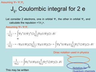
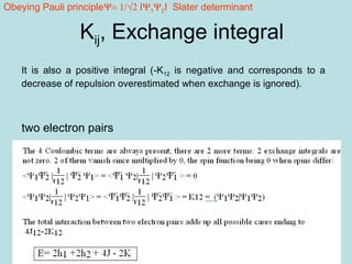
1. Hartree-Fock theory describes molecules using a linear combination of atomic orbitals to approximate molecular orbitals. It treats electrons as independent particles moving in the average field of other electrons. 2. The Hartree-Fock method involves iteratively solving the Fock equations until self-consistency is reached between the input and output orbitals. This approximates electron correlation by including an average electron-electron repulsion term. 3. The Hartree-Fock method satisfies the Pauli exclusion principle through the use of Slater determinants, which are antisymmetric wavefunctions that go to zero when the spatial or spin coordinates of any two electrons are identical.


![Polymer [ बहुलक ] Chemistry Notes PDF - Irfanullah Mehar - JJ Sir Chemistry.pdf](https://cdn.slidesharecdn.com/ss_thumbnails/polymerchemistrynotespdf-irfanullahmehar-jjsirchemistry-260210172118-3f9b37f7-thumbnail.jpg?width=640&height=640&fit=bounds)


![ANIMAL_CELL_,_TISSUE_AND_ORGAN_CULTURE[1].pptx](https://cdn.slidesharecdn.com/ss_thumbnails/animalcelltissueandorganculture1-260204172026-4462b440-thumbnail.jpg?width=640&height=640&fit=bounds)

