1) Electronic spectroscopy analyzes the energy levels of electrons in atoms.
2) Atoms consist of a positively charged nucleus surrounded by negatively charged electrons. Only certain electron orbits are allowed based on quantum mechanics.
3) The hydrogen atom has a simple structure with one electron. Its energy levels are represented by an equation involving the Rydberg constant. Transitions between levels produce spectral lines.
NQR - DEFINITION - ELECTRIC FIELD GRADIENT - NUCLEAR QUADRUPOLE MOMENT - NUCLEAR QUADRUPOLE COUPLING CONSTANT - PRINCIPLE OF NQR - ENERGY OF INTERACTION - SELECTION RULE - FREQUENCY OF TRANSITION - APPLICATIONS
In 1916, Sommerfeld extended Bohr's atomic model with the assumption of elliptical electron paths to explain the fine splitting of the spectral lines in the hydrogen atom. It is known as the Bohr-Sommerfeld model.
For more information on this concept, kindly visit our blog article at;
https://jayamchemistrylearners.blogspot.com/2022/04/bohr-sommerfeld-model-chemistrylearners.html
more chemistry contents are available
1. pdf file on Termmate: https://www.termmate.com/rabia.aziz
2. YouTube: https://www.youtube.com/channel/UCKxWnNdskGHnZFS0h1QRTEA
3. Facebook: https://web.facebook.com/Chemist.Rabia.Aziz/
4. Blogger: https://chemistry-academy.blogspot.com/
BS-III
The Aufbau Principle requires that the electrons occupy the lowest possible energy level before filling up the next.
Pauli’s Exclusion Principle posits that no two electrons can have the same set of four quantum number; the spin quantum number limits the number of electrons in an orbital to a maximum of two.
Hund’s Rule requires that the electrons fill the orbitals in a subshell one by one, before pairing the electrons in an orbital spin in opposite directions.
Read| The latest issue of The Challenger is here! We are thrilled to announce that our school paper has qualified for the NATIONAL SCHOOLS PRESS CONFERENCE (NSPC) 2024. Thank you for your unwavering support and trust. Dive into the stories that made us stand out!
How to Make a Field invisible in Odoo 17Celine George
It is possible to hide or invisible some fields in odoo. Commonly using “invisible” attribute in the field definition to invisible the fields. This slide will show how to make a field invisible in odoo 17.
Operation “Blue Star” is the only event in the history of Independent India where the state went into war with its own people. Even after about 40 years it is not clear if it was culmination of states anger over people of the region, a political game of power or start of dictatorial chapter in the democratic setup.
The people of Punjab felt alienated from main stream due to denial of their just demands during a long democratic struggle since independence. As it happen all over the word, it led to militant struggle with great loss of lives of military, police and civilian personnel. Killing of Indira Gandhi and massacre of innocent Sikhs in Delhi and other India cities was also associated with this movement.
We all have good and bad thoughts from time to time and situation to situation. We are bombarded daily with spiraling thoughts(both negative and positive) creating all-consuming feel , making us difficult to manage with associated suffering. Good thoughts are like our Mob Signal (Positive thought) amidst noise(negative thought) in the atmosphere. Negative thoughts like noise outweigh positive thoughts. These thoughts often create unwanted confusion, trouble, stress and frustration in our mind as well as chaos in our physical world. Negative thoughts are also known as “distorted thinking”.
Welcome to TechSoup New Member Orientation and Q&A (May 2024).pdfTechSoup
In this webinar you will learn how your organization can access TechSoup's wide variety of product discount and donation programs. From hardware to software, we'll give you a tour of the tools available to help your nonprofit with productivity, collaboration, financial management, donor tracking, security, and more.
The Roman Empire A Historical Colossus.pdfkaushalkr1407
The Roman Empire, a vast and enduring power, stands as one of history's most remarkable civilizations, leaving an indelible imprint on the world. It emerged from the Roman Republic, transitioning into an imperial powerhouse under the leadership of Augustus Caesar in 27 BCE. This transformation marked the beginning of an era defined by unprecedented territorial expansion, architectural marvels, and profound cultural influence.
The empire's roots lie in the city of Rome, founded, according to legend, by Romulus in 753 BCE. Over centuries, Rome evolved from a small settlement to a formidable republic, characterized by a complex political system with elected officials and checks on power. However, internal strife, class conflicts, and military ambitions paved the way for the end of the Republic. Julius Caesar’s dictatorship and subsequent assassination in 44 BCE created a power vacuum, leading to a civil war. Octavian, later Augustus, emerged victorious, heralding the Roman Empire’s birth.
Under Augustus, the empire experienced the Pax Romana, a 200-year period of relative peace and stability. Augustus reformed the military, established efficient administrative systems, and initiated grand construction projects. The empire's borders expanded, encompassing territories from Britain to Egypt and from Spain to the Euphrates. Roman legions, renowned for their discipline and engineering prowess, secured and maintained these vast territories, building roads, fortifications, and cities that facilitated control and integration.
The Roman Empire’s society was hierarchical, with a rigid class system. At the top were the patricians, wealthy elites who held significant political power. Below them were the plebeians, free citizens with limited political influence, and the vast numbers of slaves who formed the backbone of the economy. The family unit was central, governed by the paterfamilias, the male head who held absolute authority.
Culturally, the Romans were eclectic, absorbing and adapting elements from the civilizations they encountered, particularly the Greeks. Roman art, literature, and philosophy reflected this synthesis, creating a rich cultural tapestry. Latin, the Roman language, became the lingua franca of the Western world, influencing numerous modern languages.
Roman architecture and engineering achievements were monumental. They perfected the arch, vault, and dome, constructing enduring structures like the Colosseum, Pantheon, and aqueducts. These engineering marvels not only showcased Roman ingenuity but also served practical purposes, from public entertainment to water supply.
Students, digital devices and success - Andreas Schleicher - 27 May 2024..pptxEduSkills OECD
Andreas Schleicher presents at the OECD webinar ‘Digital devices in schools: detrimental distraction or secret to success?’ on 27 May 2024. The presentation was based on findings from PISA 2022 results and the webinar helped launch the PISA in Focus ‘Managing screen time: How to protect and equip students against distraction’ https://www.oecd-ilibrary.org/education/managing-screen-time_7c225af4-en and the OECD Education Policy Perspective ‘Students, digital devices and success’ can be found here - https://oe.cd/il/5yV
Instructions for Submissions thorugh G- Classroom.pptxJheel Barad
This presentation provides a briefing on how to upload submissions and documents in Google Classroom. It was prepared as part of an orientation for new Sainik School in-service teacher trainees. As a training officer, my goal is to ensure that you are comfortable and proficient with this essential tool for managing assignments and fostering student engagement.
Instructions for Submissions thorugh G- Classroom.pptx
Chapter 5 - Electronic Spectroscopy of Atoms.pdf
1. Electronic Spectroscopy of Atoms
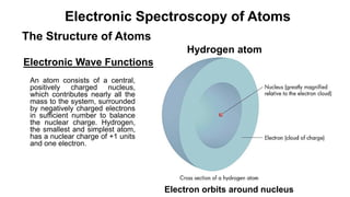
The Structure of Atoms
Electronic Wave Functions
Hydrogen atom
Electron orbits around nucleus
An atom consists of a central,
positively charged nucleus,
which contributes nearly all the
mass to the system, surrounded
by negatively charged electrons
in sufficient number to balance
the nuclear charge. Hydrogen,
the smallest and simplest atom,
has a nuclear charge of +1 units
and one electron.
5. The Energies of Atomic orbitals; Hydrogen Atom Spectrum
The energy of each orbital varies considerably from atom to atom.
There are two main contributions of this energy:
(i) Attraction between electrons and nucleus
(ii) Repulsion between electrons in the same atom.
We consider first the case of hydrogen having only one electron,
factor (ii) is completely absent. Because of the absence of
interelectronic effects all orbitals with the same n value have the
same energy in hydrogen. Thus the 2s and 2p orbitals are
degenerate as are the 3s, 3p and 3d. However, the energies of the
2s, 3s, 4s, … orbitals differ considerably. For the s orbitals given
by the following equation:
𝝍𝑛𝑠= ƒ
𝑟
𝑎0
exp −
𝑟
𝑛𝑎0
6. The Schrödinger equation shows that the energy is:
𝐸𝑛 = −
𝑚𝑒4
8ℎ2𝜀0
2𝑛2 J
(1)
𝜀𝑛 = −
𝑚𝑒4
8ℎ3𝑐𝜀0
2𝑛2 = −
𝑅
𝑛2 cm‒1 (n = 1, 2, 3, …..)
Where ɛ0 is the vacuum permittivity and where the fundamental constants
have been collected together and given the symbol R, called the Rydberg
constant. Since p, d, …. orbitals have the same energies as the corresponding
s (for hydrogen only), Eq. (1) represents all the electronic energy levels of this
atom.
The lowest value of ɛn is plainly ɛn = ‒R cm‒1 (when n = 1), and so this
represents the most stable (or ground) state; ɛn increases with increasing n,
reaching a limit, ɛn = 0 for n = ∞. This represents complete removal of the
electron from the nucleus, i.e. the state of ionization. We sketch these energy
levels for n = 1 to 5 and l = 0, 1, and 2 only in Fig. ….
7. Figure: Some of the lower electronic energy
levels and transitions between them for the
single electron of the hydrogen atom.
Equation (1) and Figure represent the
energy levels of the atom. The Schrödinger
equation shows these to be:
Δn = anything and Δl = ±1 only (2)
From these selection rules we see
immediately that an electron in the ground
state (the 1s) can undergo a transition into
any p state:
1s → np (n ≥ 2)
While a 2p electron can have transitions
either into an s or a d state:
2p → ns or nd
Since s and d orbitals are here degenerate
the energy of both these transitions will be
identical. These transitions are sketched in
this Figure.
8.
9. Figure: Representation of part of
the Lyman series of the hydrogen
atom, showing the convergence
(ionization) point.
11. Electronic Angular Momentum
Orbital Angular Momentum
An electron moving in its orbital about a nucleus possesses orbital angular
momentum, a measure of which is given by the l value corresponding to the
orbital. This momentum is quantized and it is usually expressed in terms of
the unit h/2π, where h is Planck’s constant. We may write:
Orbital angular momentum = 𝑙(𝑙 + 1).
ℎ
2𝜋
= 𝑙(𝑙 + 1) units (3)
The orbital angular momentum is represented by the symbol I where:
I = 𝑙(𝑙 + 1) units (4)
12. Figure: The allowed directions of the electronic momentum
vector for an electron in (a) a p state (l = 1), (b) a d state (l =
2) and (c) the allowed directions of the electronic spin
angular momentum vector. The reference direction is taken
arbitrarily as upwards in the plane of the paper.
Figure (a) and (b) shows the situation for
an electron with l = 1 and l = 2,
respectively (i.e. a p and a d electron).
The reference direction is conventionally
used to define the z axis, and so we can
write the components of I in this direction
as Iz.
Iz = lz ·
ℎ
2𝜋
(5)
lz = l, l – 1,..., 0, …, –(l – 1), l (6)
And that there are 2l+1 values of lz for a
given l. Plainly lz is to be identified with
the magnetic quantum number m
introduced by
lz ≡ m
13. Electron Spin Angular Momentum
Every electron in an atom can be considered to be spinning about an axis
as well as orbiting about the nucleus. Its spin motion is designated by the
spin quantum number s , which can be shown to have a value
1
2
only.
Thus the spin angular momentum is given by:
s = 𝑠 𝑠 + 1
ℎ
2𝜋
=
1
2
×
3
2
units (7)
=
1
2
3 units
The quantization law for spin momentum is that the vector can point so as
to have components in the reference direction which are half-integral
multiples of h/2π, i.e. so that sz = szh/2π with sz taking values +
1
2
𝑜𝑟 −
1
2
only. The two (that is 2s + 1) allowed directions are shown in previous
Figure (c); they are normally degenerate.
14. Total Electronic Angular Momentum
The orbital and spin contributions to the electronic angular momentum may be combined. Formally we can write:
j = I + s (8)
where j is the total angular momentum. Since I and s are vectors, Eq. (8) must be taken to imply vector addition.
Also formally, we can express j in terms of a total angular momentum quantum number j:
j = 𝑗 𝑗 + 1
ℎ
2𝜋
= 𝑗(𝑗 + 1) units (9)
where j is half-integral and a quantal law applies equally to j as to I and s: j can have z-components which are
half-integral only i.e.:
jz = ±j, ±(j – 1), ±(j – 2), …..,
1
2
(10)
There are two methods by which we can deduce the various allowed values of j for particular I and s values.
(1) Vector summation: l = 1, s =
1
2
and hence j = l + s =
3
2
or j = l – s =
1
2
Figure: The two energy states having
different total angular momentum which
can arise as a result of the vector addition
of I = 2 and s =
1
2
3.
(2) Summation of z components: jz= lz + sz
15. The Fine Structure of the Hydrogen Atom Spectrum
Figure: Some of the lower energy levels of the hydrogen
atom showing the inclusion of j-splitting. The splitting is
greatly exaggerated for clarity.
Each level is labelled with its n quantum
number on the extreme left and its j value on
the right; the l value is indicated by the state
symbols S, P, D, … at the top of each column.
It suggests that the j-splitting decreases with
increasing n and with increasing l.
The selection rules for n and l are:
Δn = anything Δl = ±1 (11)
but now there is a selection rule for j:
Δj = 0, ±1 (12)
These selection rules indicate that transitions
are allowed between any S level and any P
level:
2S1/2 → 2P1/2 (Δj = 0)
2S1/2 → 2P3/2 (Δj = +1)
16. Transition between the 2P and 2D states are
rather more complex. Figure shows four of the
energy levels involved. Plainly the transition at
lowest frequency will be that between the
closest pair of levels, the 2P3/2 and 2D3/2. This,
corresponding to Δj = 0 is allowed. The next
transition, 2P3/2 → 2D5/2 (Δj = +1), is also allowed
and will occur close to the first because the
separation between the doublet D states is very
small. Thirdly, and more widely spaced, will be
2P1/2 → 2D3/2 (Δj = +1), but the forth transition
(shown dotted) 2P1/2 → 2D5/2, is not allowed
since for this Δj = +2. Thus the spectrum will
consist of the three lines shown at the foot of
the figure. This is usually referred to as a
compound doublet spectrum.
Figure: The ‘compound doublet’ spectrum arising as the
result of transitions between 2P and 2D levels in the
hydrogen atom.
17. Many-Electron Atoms
The Building-Up Principle
The Schrödinger equation shows that electrons in atoms occupy orbitals of the same type and shape as
the s, p, d, …… orbitals discussed for the hydrogen atom, but that the energies of these electrons differ
markedly from atom to atom. There are three basic rules, known as the building-up rules, which
determine how electrons in large atoms occupy orbitals. These may be summarized as:
1. Pauli’s principle: no two electrons in an atom may have the same set of values for n, l, Iz (≡ m), and sz.
2. Electrons tend to occupy the orbital with lowest energy available.
3. Hund’s principle: electrons tend to occupy degenerate orbitals singly with their spins parallel.
Electronic structure of some atoms
We may write the n, l, Iz and sz values as:
18. The Spectrum of Lithium and Other Hydrogen-Like Species
Figure: Some of the lower energy levels of the lithium
atom, showing the difference in energy of s, p, and d
states with the same value of n. Some allowed transitions
are also shown. The j-splitting is greatly exaggerated.
The energy levels of lithium are sketched in Figure.
The selection rules for alkali metals are the same as
for hydrogen, that is Δn = anything, Δl = ±1, Δj = 0, ±1
and so the spectra will be similar also. Thus transitions
from the ground state (1s22s) can occur to p levels:
2S1/2 → nP1/2,3/2, and a series of doublets similar to the
Lyman series will be formed, converging to some point
from which the ionization potential can be found. From
the 2p state, however, two separate series of lines will
be seen:
2 2P1/2, 3/2 → n 2S1/2
and 2 2P1/2, 3/2 → n 2D3/2, 5/2
The former will be doublets, the latter compound
doublets, but their frequencies will differ because the s
and d orbital energies are no longer the same.
19. The Angular Momentum of Many-Electron Atoms
There are two different ways in which we might sum the orbital and spin momentum
of several electrons:
1. First sum the orbital contributions, then the spin contributions separately, and
finally add the total orbital and
total spin contributions to reach the grand total. Symbolically:
𝐈𝑖 = 𝐋 𝐬𝑖 = 𝐒 L + S = J
where we use bold-face capital letters to designate total momentum.
2. Sum the orbital and spin momenta of each electron separately, finally summing
the individual totals to form
the grand total:
Ii + si = ji 𝐣𝑖 = 𝐉
The first method, Known as Russell-Saunders coupling, gives results in accordance
with the spectra of small and medium-sized atoms, while the second (called j-j
coupling, since individual j’s are summed) applies better to large atoms.
20. Summation of Orbital Contributions
The orbital momenta I1, I2, …. of several electrons may be added by the same methods as the
summation of the orbital and spin momenta of a single electron. Thus we could:
1. Add the vectors I1, I2, ….. Graphically, remembering that their resultant L must
be expressible by:
𝐋 = 𝐿(𝐿 + 1) (L = 0, 1, 2, …..) (13)
where L is the total momentum quantum number. Thus L can have values 0, 2 , 6 , 12 , ….. only.
Figure: Summation of orbital angular momenta for a p and a d electron.
Figure illustrates the method for a p
and a d electron, l1 = 1, l2 = 2; hence
I1 = 2 , I2 = 6 . There are three
ways in which the two vectors may
be combined to give L consistent
with Eq (13). The three values of L
are seen to be 12 , 6 , and 2 ,
corresponding to the quantum
numbers L = 3, 2, and 1,
respectively.
21. 2. Alternatively, we could add the individual quantum numbers l1 and l2 to obtain the total quantum
number L according to :
L = l1 + l2, l1 + l2 – 1, …. 𝑙1 − 𝑙2 (14)
where the modulus sign … indicates that we are to take l1 – l2 or l2 – l1, whichever is positive.
For two electrons, there will plainly be 2li + 1 different values of L, where li is the smaller of the
two l values.
3. Finally we could add the z components of the individual vectors, picking out from the result sets
of components corresponding to the various allowed L values. Symbolically this process is:
𝑳𝑧 = 𝒍𝑖𝑧
22. Summation of Spin Contributions
The total spin angular momentum denoted as S and the total spin quantum number denoted as S,
we can have:
1. Graphical summation, provided the resultant is
𝐒 = 𝑆(𝑆 + 1) (15)
where S is either integral or zero only, if the number of contributing spins is even, or half-integral
only, if the number is odd,
2. Summation of individual quantum numbers. For N spins we have:
S = 𝑠𝒊, 𝑠𝑖 − 1, 𝑠𝑖 − 2, …..
=
𝑁
2
,
𝑁
2
− 1, ….,
1
2
(for N odd) (16)
=
𝑁
2
,
𝑁
2
− 1, …., 0 (for N even)
3. Summation of individual sz to give Sz.
Method 2, which is always applicable and simple. Thus for two electrons we have the two possible
spin states:
S =
1
2
+
1
2
= 1 or S =
1
2
+
1
2
− 1 = 0
In the former the spins are called parallel and the state may be written (↑↑), while in the latter they
are paired or opposed and written (↑↓).
23. Again, for three electrons we may have:
S =
1
2
+
1
2
+
1
2
=
3
2
(↑↑↑)
S =
1
2
+
1
2
+
1
2
− 1 =
1
2
(↑↑↓, ↑↓↑, or ↓↑↑)
where we see that there are three ways in
which the S =
1
2
state may be realized and
one in which S =
3
2
.
Figure: The z components of (a) an orbital angular
momentum vector, (b) a spin vector for which S is half-
integral, and (c) a spin vector for which S is integral.
24. Total Angular Momentum
The addition of the total orbital momentum L and the total spin momentum S to give the grand
total momentum J can be carried out in the same ways as the addition of l and s to give j, for a
single electron. The only additional point is that the quantum number J in the expression:
J = 𝐽 𝐽 + 1
ℎ
2𝜋
(17)
must be integral if S is integral and half-integral if S is half-integral. In terms of the quantum
numbers we can write immediately:
J = L + S, L + S – 1, …., 𝐿 − 𝑆 (18)
Where, as before, the positive value of L – S, is the lowest limit of the series of values. For
example if L = 2, S =
3
2
, we would have:
𝐽 =
7
2
,
5
2
,
3
2
, and
1
2
while if L = 2, S = 1, the J values are:
𝐽 = 3, 2, or 1 only
25. Term Symbols
The vector quantities L, S, and J for a system may be expressed in terms of quantum numbers
L, S, and J:
L = 𝐿 𝐿 + 1 S = 𝑆 𝑆 + 1 J = 𝐽 𝐽 + 1 (19)
where the integral L and integral or half-integral S and J are themselves combinations of
individual electronic quantum numbers.
The term symbol for a particular atomic state is written as follows:
Term symbol = 2S+1LJ (20)
where the numerical superscript gives the multiplicity of the state, the numerical subscript gives
the total angular momentum number J, and the value of the orbital quantum number L is
expressed by a latter:
For L = 0, 1, 2, 3, 4, ….
Symbol = S, P, D, F, G, …..
a symbolism which is comparable with the s, p, d, …. already used for single-electron states with
l = 0, 1, 2, …..
26. Let us now see some examples.
1. S =
1
2
, L = 2; hence J =
5
2
or
3
2
and 2S + 1 = 2. Term symbols: 2D5/2 and 2D3/2, which are to be
read ‘doublet D five halves’ and ‘doublet D three halves’, respectively.
2. S = 1, L = 1; hence J = 2, 1, 0 and 2S + 1 = 3. Term symbols: 3P2, 3P1 or 3P0 (read ‘triple P
two’, etc.).
In both these examples we see that (since L ≥ S), the multiplicity is the same as the number of
different states.
3. S =
3
2
, L = 1; hence J =
5
2
,
3
2
, or
1
2
and 2S + 1 = 4. Term symbols: 4P5/2, 4P3/2, 4P1/2 (read ‘quartet
P five halves’ etc.) where, since L < S, there are only three different energy states but each is
nonetheless described as quartet since 2S + 1 = 4.
The reverse process is equally easy; given a term symbol for a particular atomic state we can
immediately deduce the various total angular momenta of that state. Some examples:
4. 3S1: we read immediately that 2S + 1 =3, and hence S = 1, and that L = 0 and J = 1.
5. 2P3/2: L = 1, J =
3
2
, 2S + 1 = 2; hence S =
1
2
.
27. The Spectrum of Helium and the Alkaline Earths
Helium consists of a central nucleus and two outer electrons. Clearly there are only two
possibilities for the relative spins of the two electrons:
1. Their spins are paired; in which case if s1 is +
1
2
, s2 must be ‒
1
2
; hence Sz = s1 + s2 = 0, and
so S = 0 and we have singlet states.
2. Their spins are parallel; now s1 = s2 = +
1
2
, say, so that Sz = 1 and their states are triplet.
The lowest possible energy state of this atom is when both electrons occupy the 1s orbital; this,
by Pauli’s principle, is possible only if their spins are paired, so the ground state of helium must
be a singlet state. Further, L = l1 + l2 = 0, and hence J can only be zero. The ground state of
helium is 1S0.
The relevant selection rules for many-electron systems are:
ΔS = 0 ΔL = ±1 ΔJ = 0, ±1 (21)
We see immediately that the singlet ground state can undergo transitions only to other singlet
states. The selection rules for L and J are the same as those for l and j considered earlier.
28. Figure: Some of the energy levels of the
electrons in the helium atom, together with a few
allowed transitions.
The left-hand side of Figure shows the energy
levels for the various singlet states which arise.
Initially the 1s2 1S0 state can undergo a transition
only to 1s1 np1 states; in the latter L = 1, S = 0,
and hence J = 1 only, so the transition may be
symbolized:
1s2 1S0 → 1snp 1P1
or, briefly:
1S0 → 1P1
From the 1P1 state the states, as shown in the
figure, or undergo transitions to the higher 1D2
states.
The right-hand side of Figure shows the energy
levels for the various triplet states.
The 1s2s state has S = 1, L = 0, and hence J = 1 only, and so it is 3S1; by the selection rules of Eq. (21) it can only
undergo transitions into the 1snp triplet states. These, with S = 1, L =1, have J = 2, 1, or 0, and so the transitions
may be written. 3S1 → 3P2, 3P1, 3P0
All three transitions are allowed, since ΔJ = 0 or ±1, so the resulting spectral lines will be triplet.
29. Figure: The ‘compound triplet’
spectrum arising from
transitions between 3P and 3D
levels in the helium atom. The
separation between levels of
different J is much exaggerated.
The Figure shows a transition between 3P and 3D states,
bearing in mind the selection rule ΔJ = 0, ±1. We note that 3P2
can go to each of 3D3,2,1, 3P1 can go only to 3D2,1, and 3P0 can
go only to 3D1. Thus the complete spectrum should consists of
six lines.
31. The high temperature of the flame excites a valence electron
to a higher-energy orbital.
The atom then emits energy in the form of light as the
electron falls back into the lower energy orbital (ground state).
The intensity of the absorbed light is proportional to the
concentration of the element in the flame.
33. Each element has a characteristic spectrum.
Example: Na gives a characteristic line at 589 nm.
Atomic spectra feature sharp bands.
There is little overlap between the spectral lines of different elements.
34.
35. Atomic absorption spectroscopy and atomic
emission spectroscopy are used to determine the
concentration of an element in solution.
36. Applying Lambert-Beer’s law in atomic absorption
spectroscopy is difficult due to
variations in the atomization from the sample matrix
non-uniformity of concentration and path length of analyte atoms.
Concentration measurements are usually determined from a
calibration curve generated with standards of known
concentration.
38. Light Source
Hollow-cathode lamp: The cathode
contains the element that is analyzed.
Atomization
Desolvation and vaporization of ions or atoms in a sample:
high-temperature source such as a flame or graphite furnace
Flame atomic absorption spectroscopy
Graphite furnace atomic absorption spectroscopy
40. Process in a Flame AA
M* M+ + e_
Mo M*
MA Mo + Ao
Solid Solution
Ionization
Excitation
Atomization
Vaporization
41. Graphite Furnace Atomic Absorption Spectroscopy
Sample holder: graphite tube
Samples are placed directly in the
graphite furnace which is then
electrically heated.
Beam of light passes through the
tube.
42. Basic Graphite Furnace Program
THGA
Three stages:
1. drying of sample
2. ashing of organic matter
3. vaporization of analyte atoms
to burn off organic
species that would
interfere with the
elemental analysis.
transversely heated graphite atomizer
45. Graphite Flame
Advantages Solutions, slurries and solid samples
can be analyzed.
Much more efficient atomization
greater sensitivity
Smaller quantities of sample
(typically 5 – 50 µL)
Provides a reducing environment for
easily oxidized elements
Inexpensive (equipment, day-
to-day running)
High sample throughput
Easy to use
High precision
Disadvantages Expensive
Low precision
Low sample throughput
Requires high level of operator skill
Only solutions can be
analyzed
Relatively large sample
quantities required (1 – 2 mL)
Less sensitivity (compared to
graphite furnace)
46. water analysis (e.g. Ca, Mg, Fe, Si, Al, Ba content)
food analysis; analysis of animal feedstuffs ( e.g. Mn,
Fe, Cu, Cr, Se, Zn)
analysis of additives in lubricating oils and greases
(Ba, Ca, Na, Li, Zn, Mg)
analysis of soils
clinical analysis (blood samples: whole blood, plasma,
serum; Ca, Mg, Li, Na, K, Fe)
Applications of Atomic Absorption Spectroscopy