Downloaded 189 times


![4
SPATIAL DOMAIN
• Procedures that operate
directly on pixels.
g(x,y) = T[f(x,y)]g(x,y) = T[f(x,y)]
where
– f(x,y)f(x,y) is the input image
– g(x,y)g(x,y) is the processed image
– TT is an operator on ff defined
over some neighborhood of
(x,y)(x,y)](https://image.slidesharecdn.com/spatialdomainandfiltering-161130205601/75/Spatial-domain-and-filtering-4-2048.jpg)


![IMAGE ENHANCEMENT IN THE
SPATIAL DOMAIN
(HISTOGRAM PROCESSING)
Intensity distribution in the image
The histogram functions count the number
of elements within a range and display each range
as a rectangular bin. The height (or length
when using rose) of the bins represents the
number of values that fall within each range.
for (int i=0;i<width;i++){
for (int j=0;j<height;j++){
int x = pixels[i][j];
histData[x] =histData[x]+1;
}
}
November 30, 2016 10](https://image.slidesharecdn.com/spatialdomainandfiltering-161130205601/75/Spatial-domain-and-filtering-10-2048.jpg)
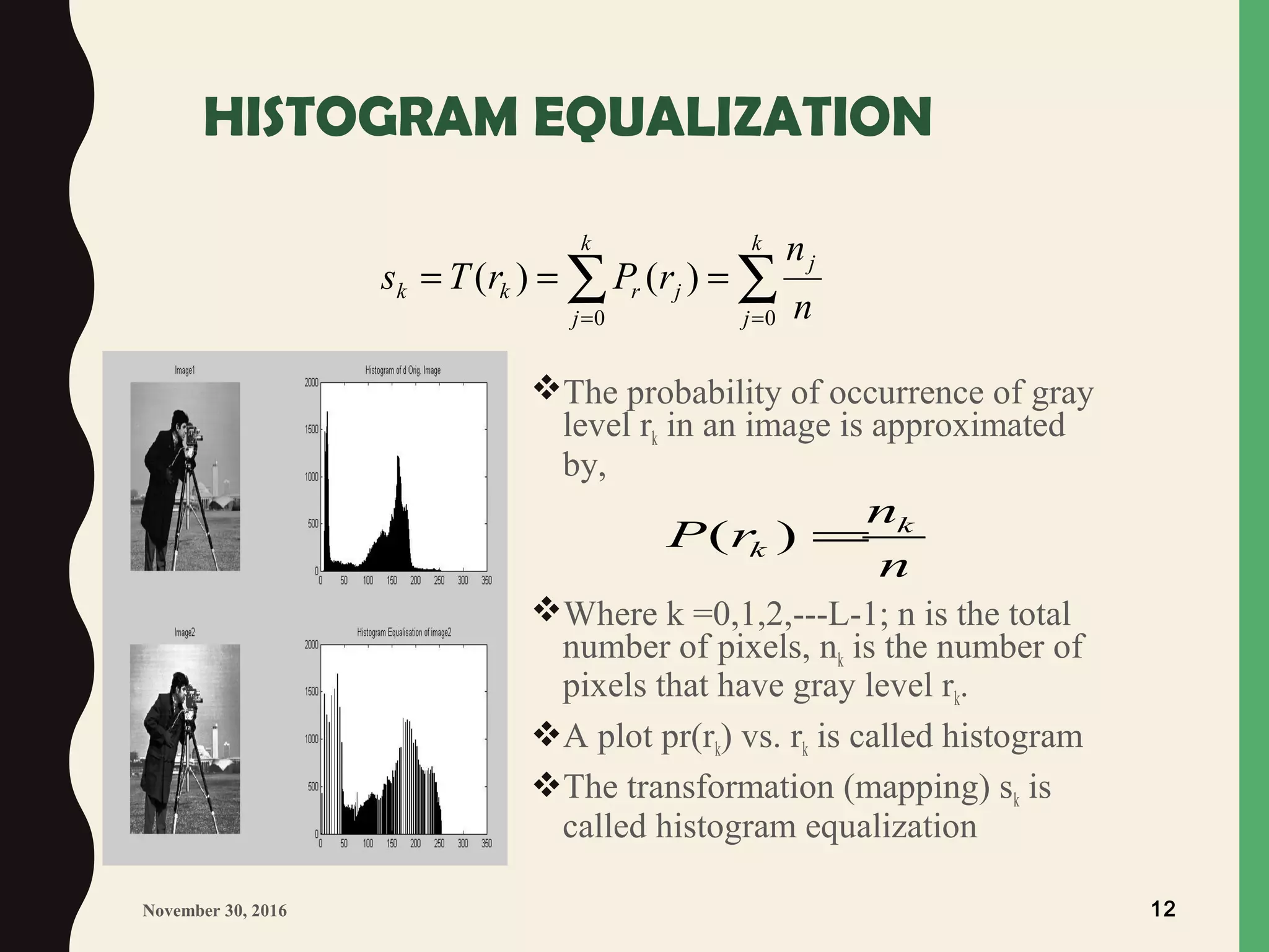
![HISTOGRAM EQUALIZATION ALGORITHM
1. Calculate Histogram
loop over i ROWS of input image
loop over j COLS of input image
k = input_image[i][j]
hist[k] = hist[k] + 1
end loop over j
end loop over i
2. calculate the sum of hist
loop over i gray levels
sum = sum + hist[i]
sum_of_hist[i] = sum
end loop over i
November 30, 2016 13
3. Transform input image to
output image
area = area of image (ROWS x COLS)
Dm = number of gray levels in output
image
loop over i ROWS
loop over j COLS
k = input_image[i][j]
out_image[i][j] = (Dm/area) x sum_of_hist[k]
end loop over j
end loop over i](https://image.slidesharecdn.com/spatialdomainandfiltering-161130205601/75/Spatial-domain-and-filtering-13-2048.jpg)
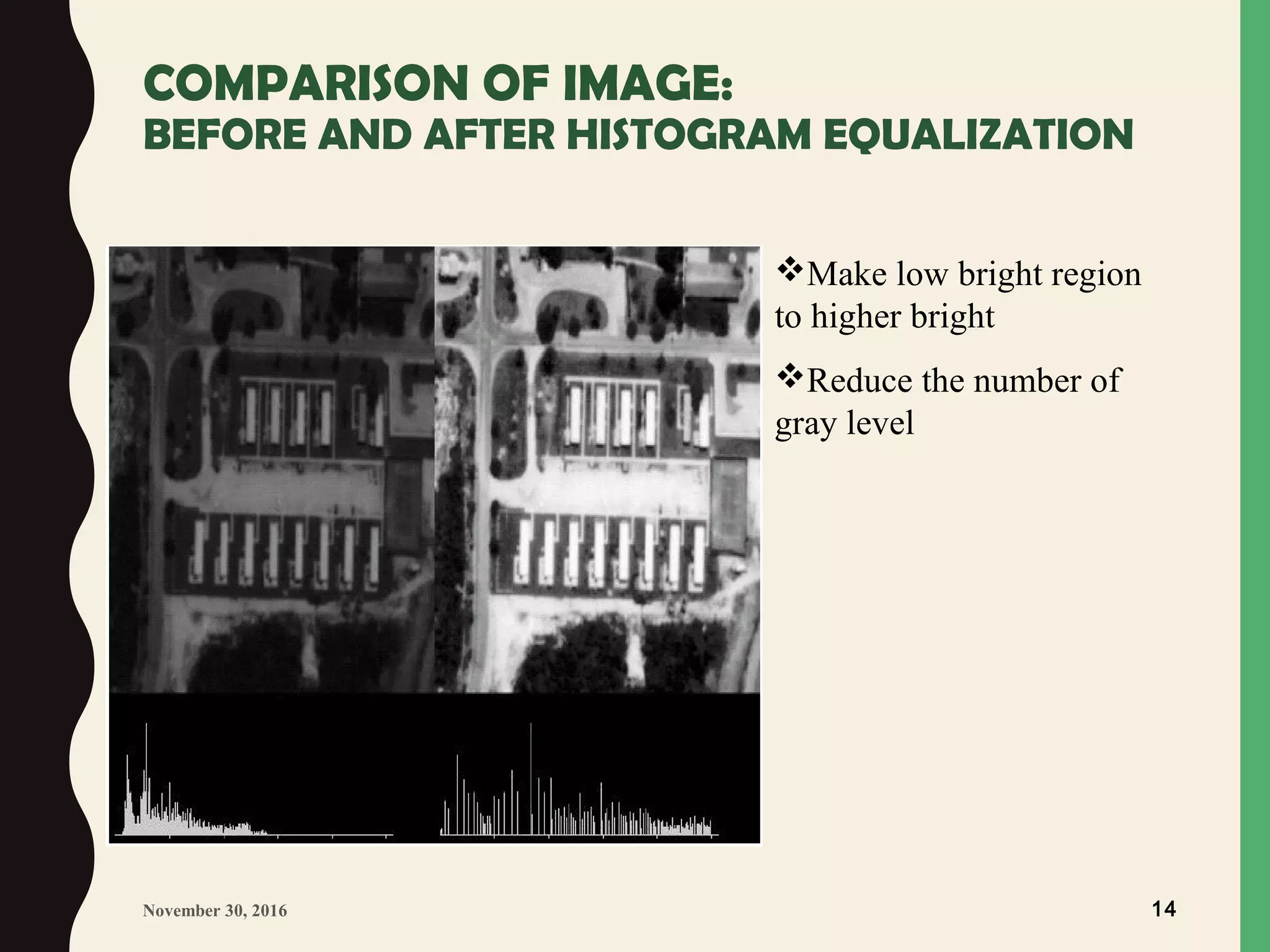
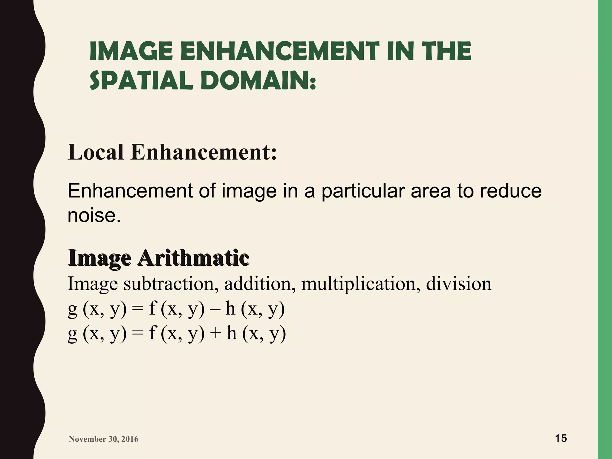
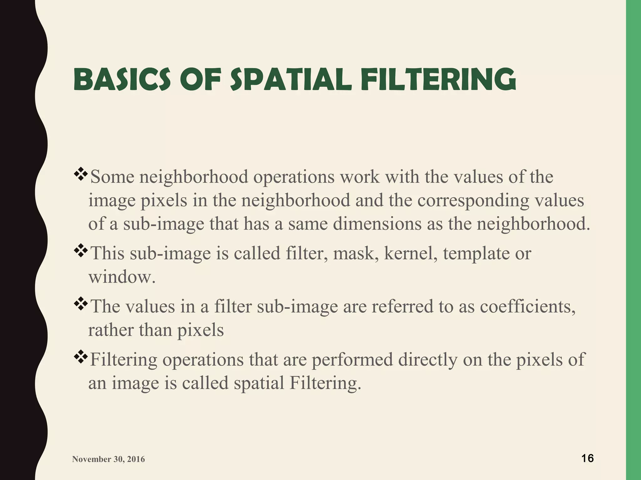


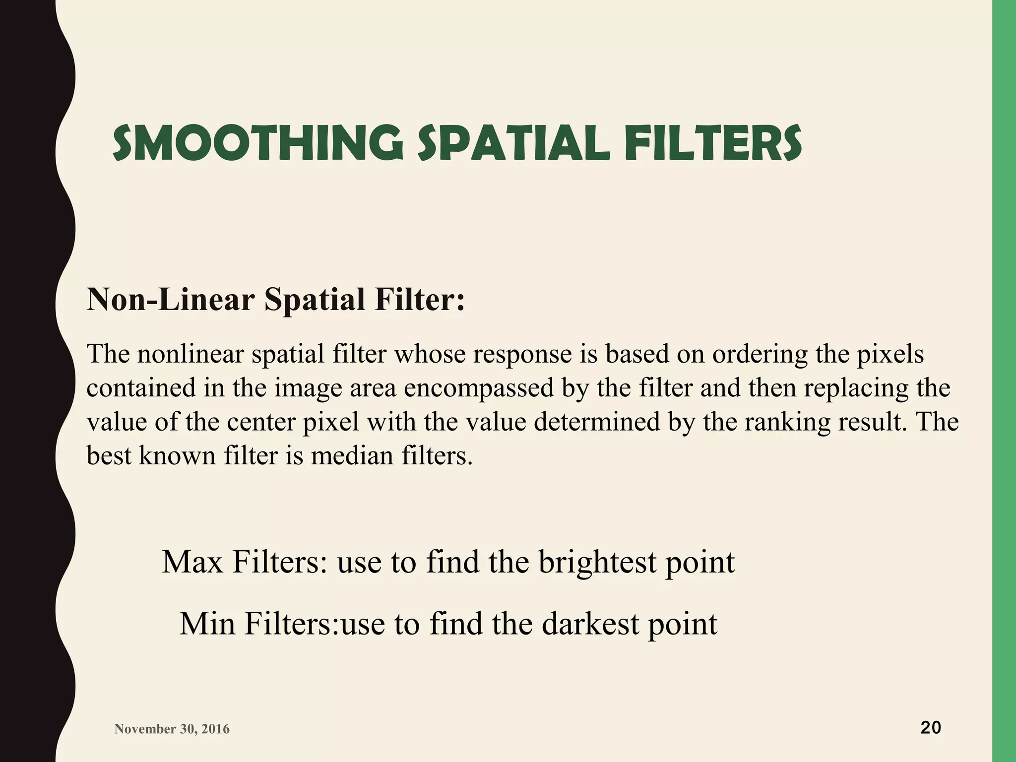


The document discusses image enhancement techniques in digital image processing, focusing on spatial domain methods. It covers various approaches like contrast stretching, histogram processing, and spatial filtering, explaining mechanisms such as pixel manipulation and the application of filters. Additionally, it distinguishes between linear and non-linear filtering techniques and their roles in enhancing image quality.