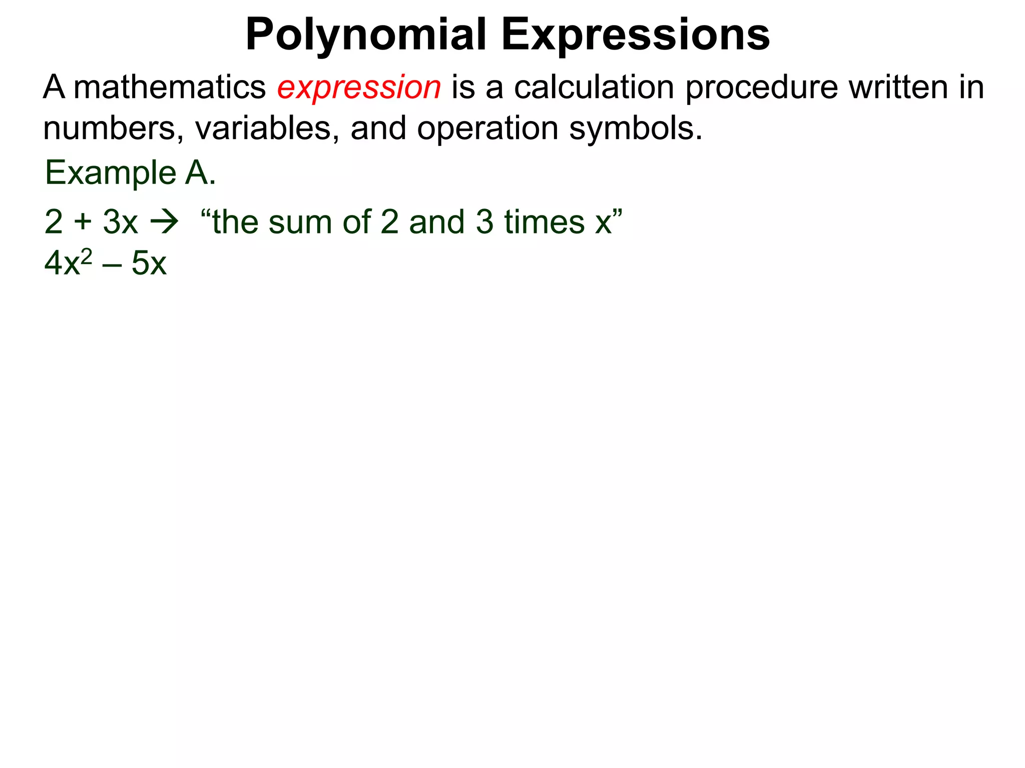
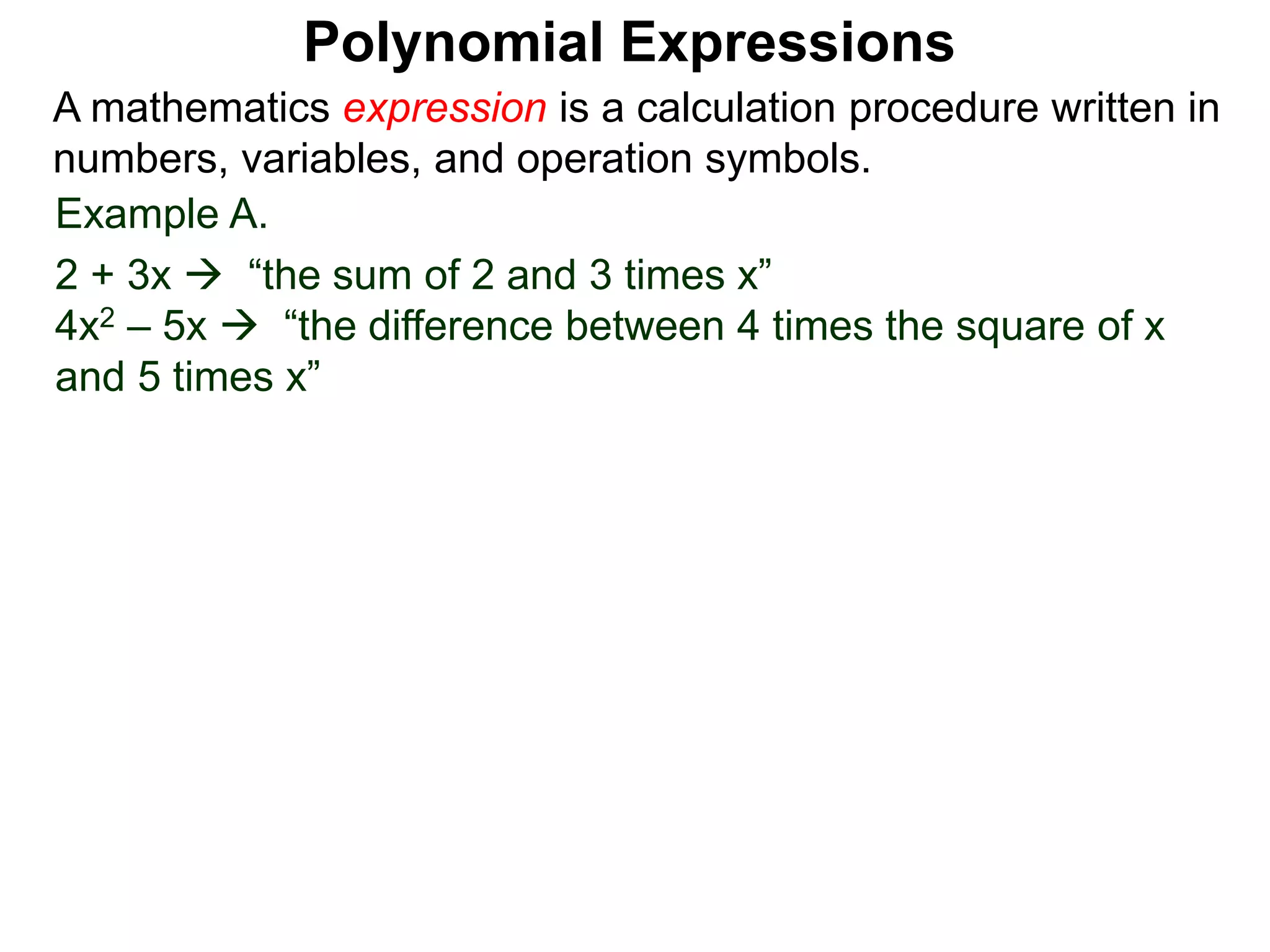
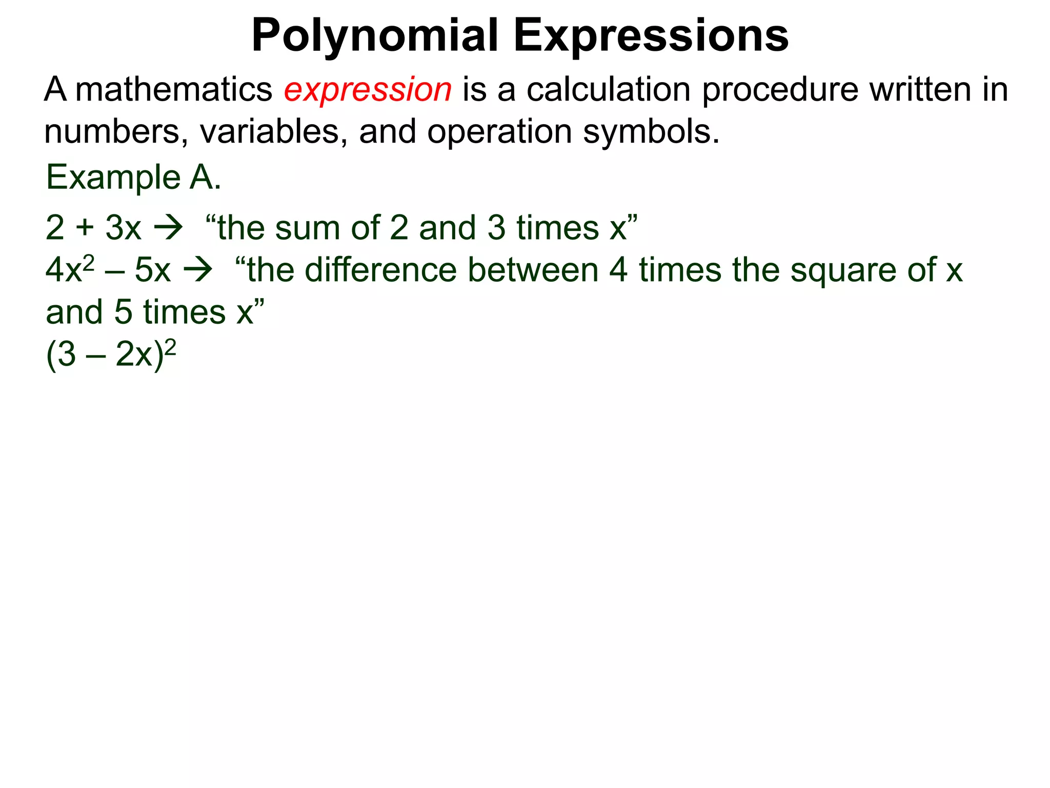
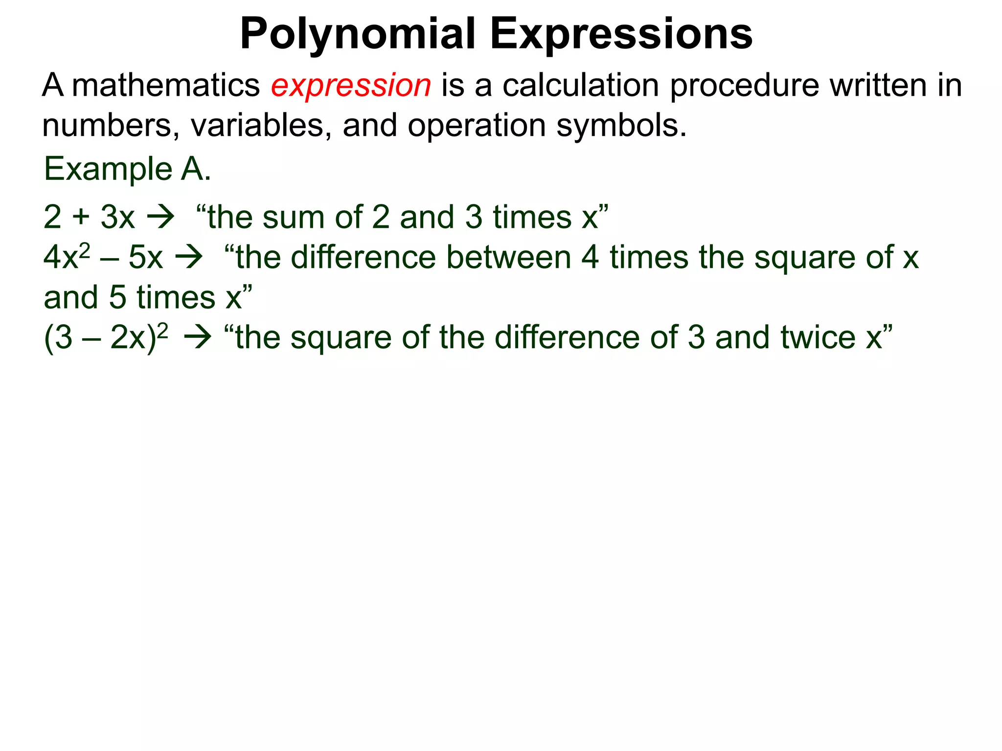
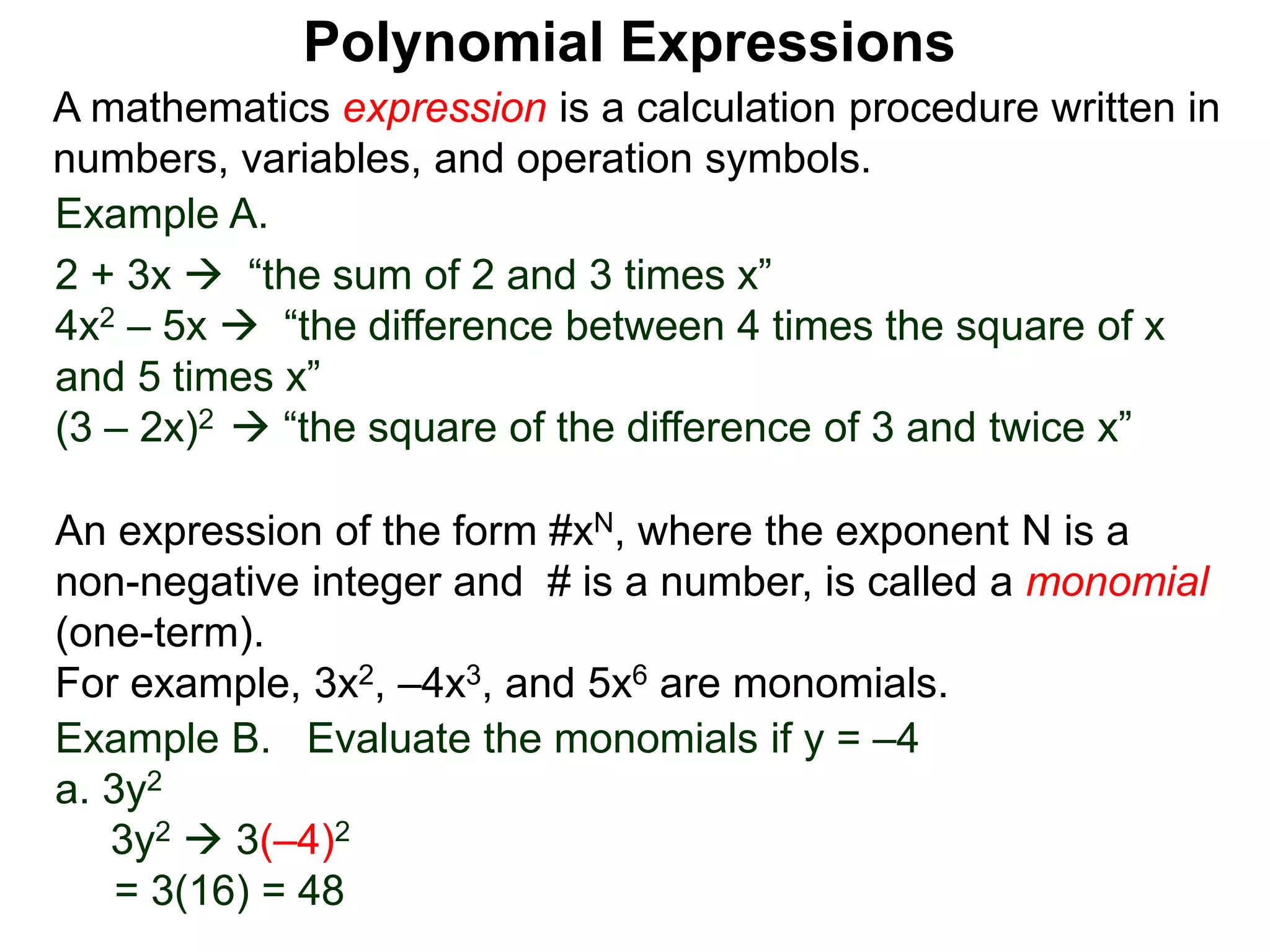
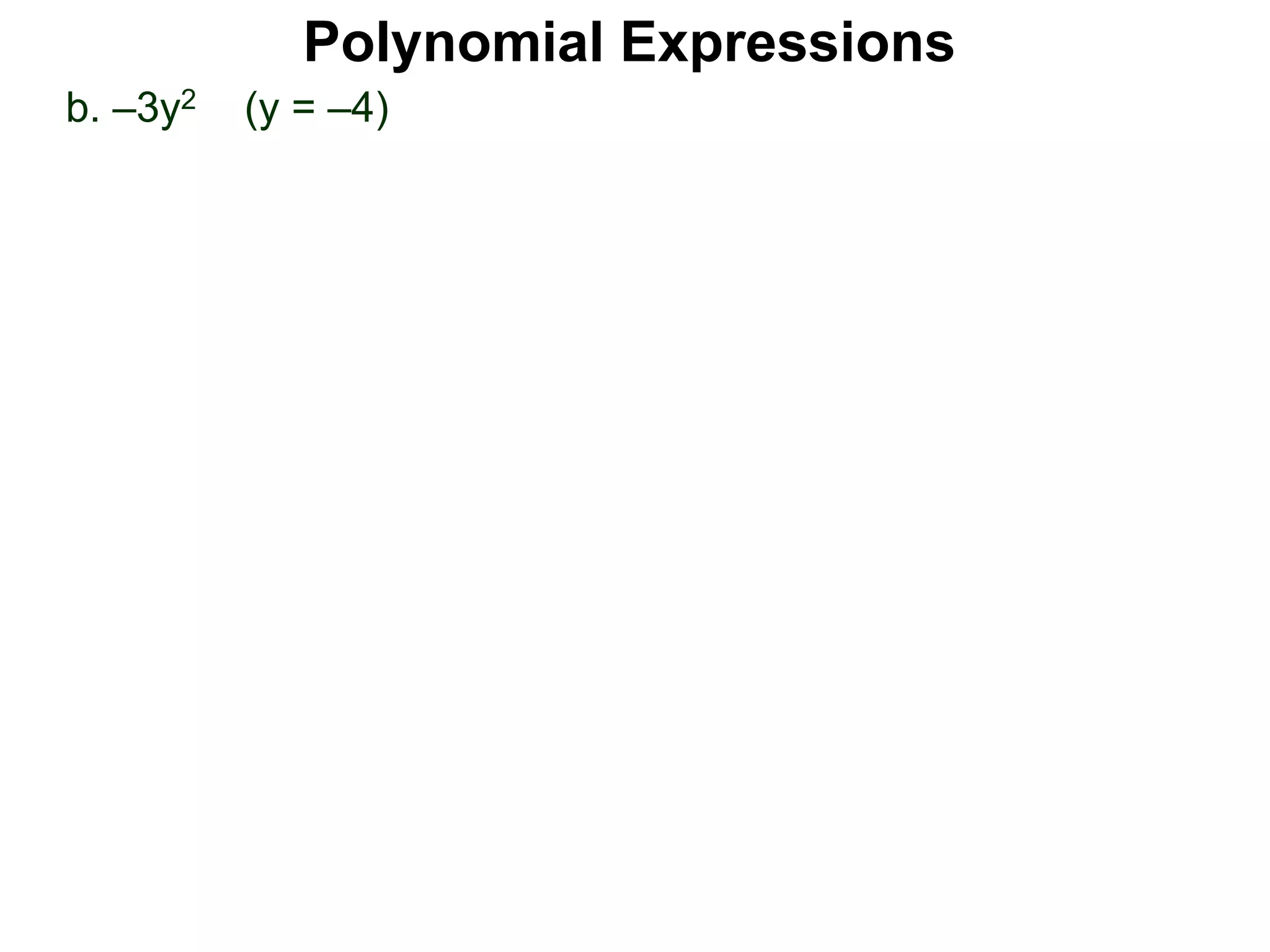
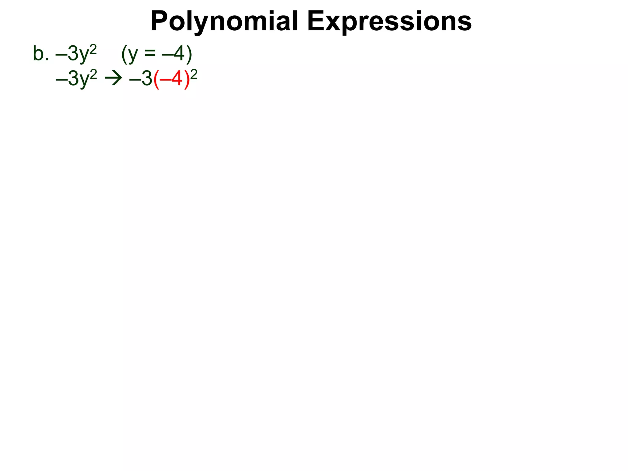
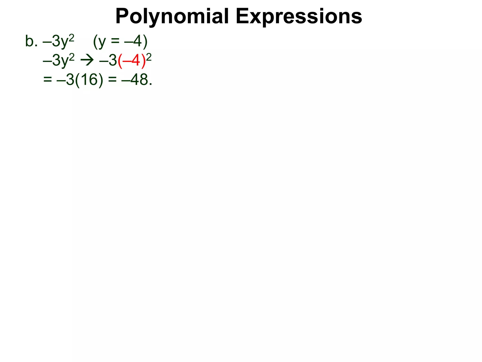
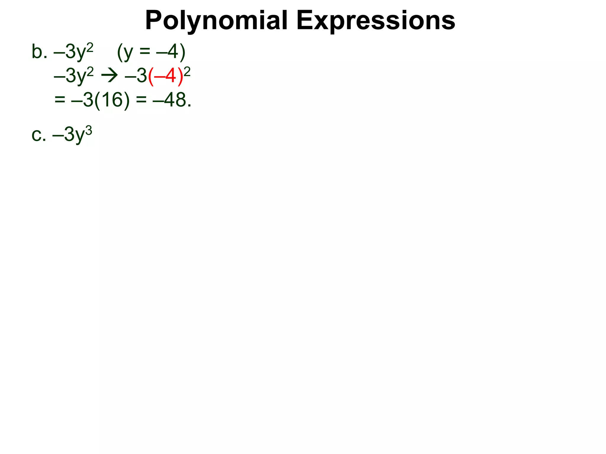
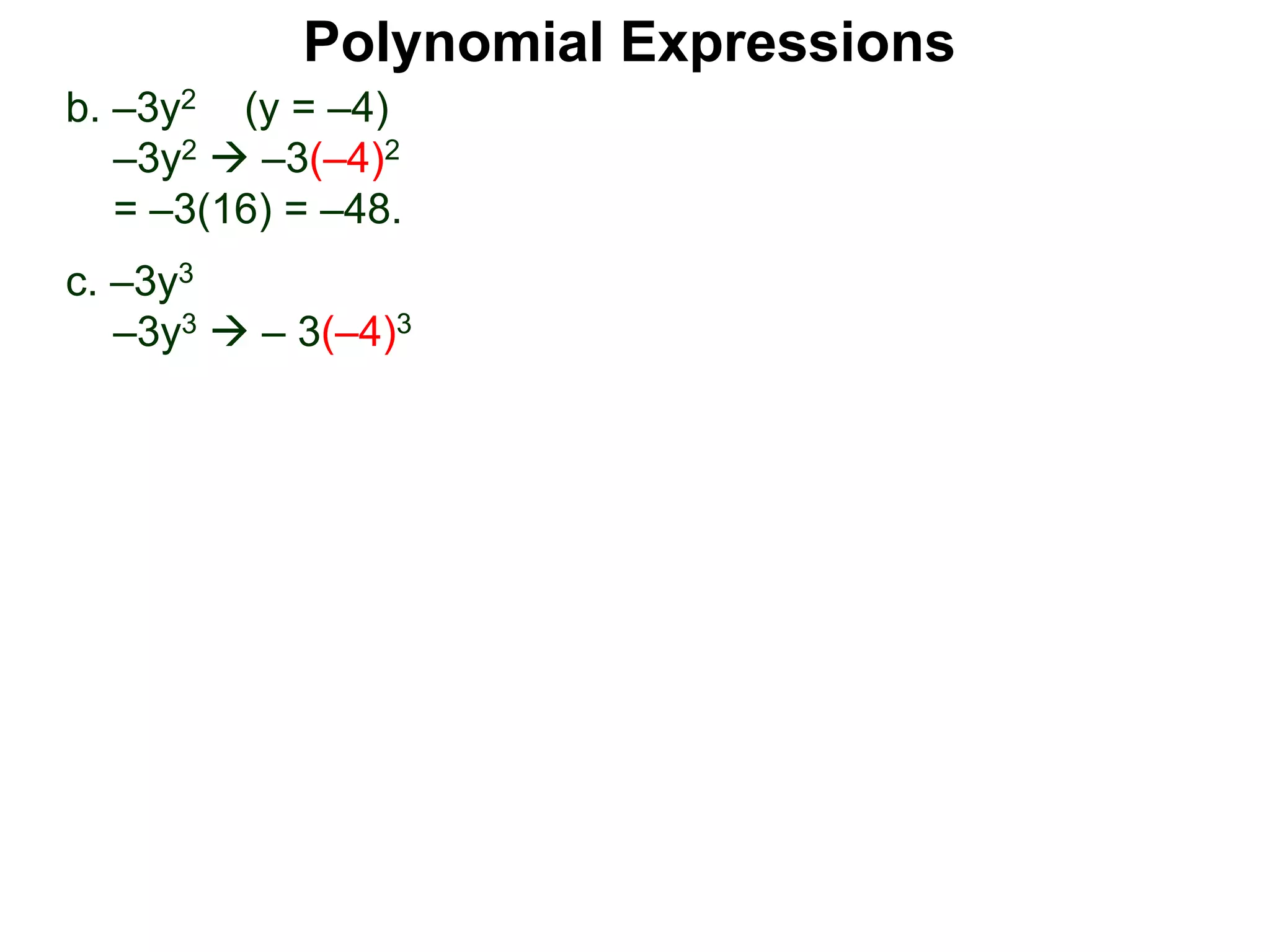
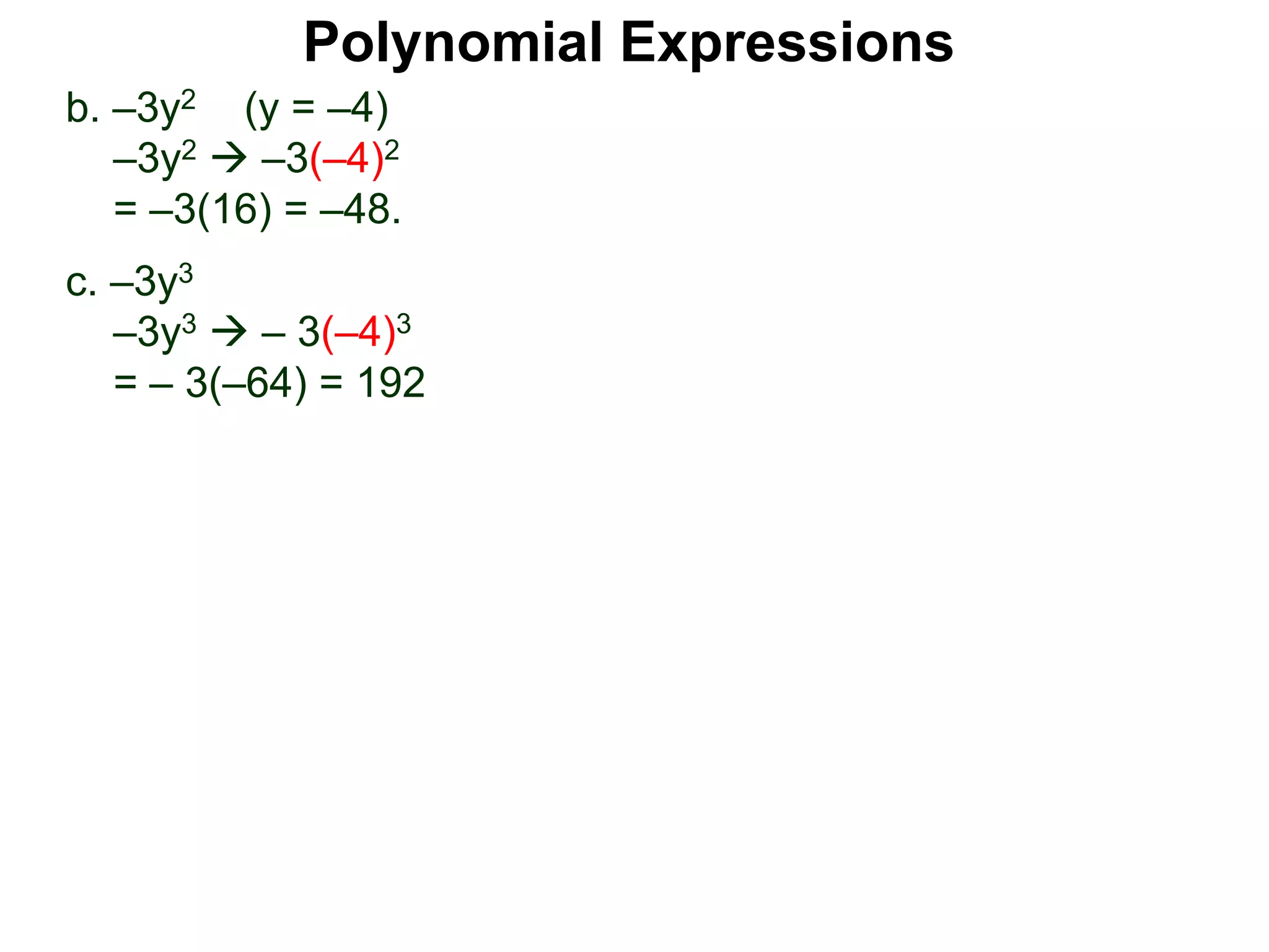
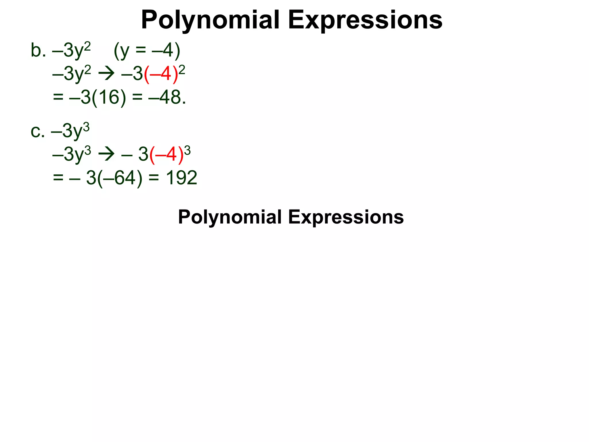
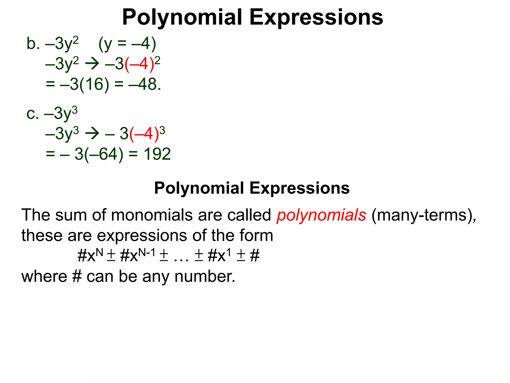
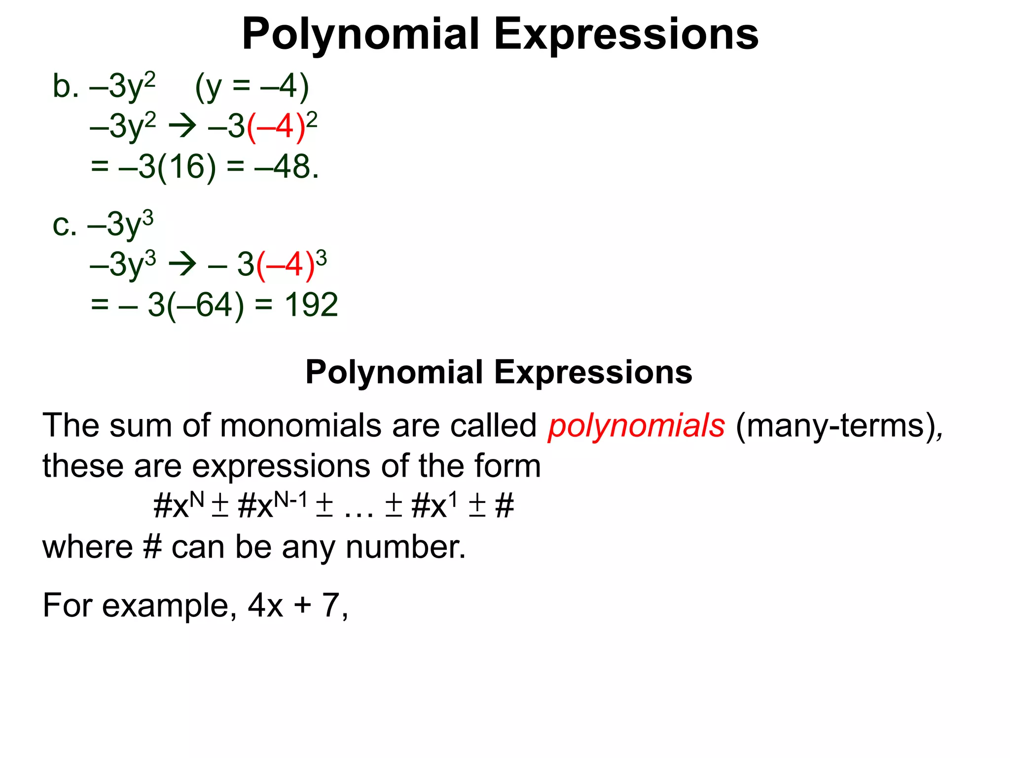
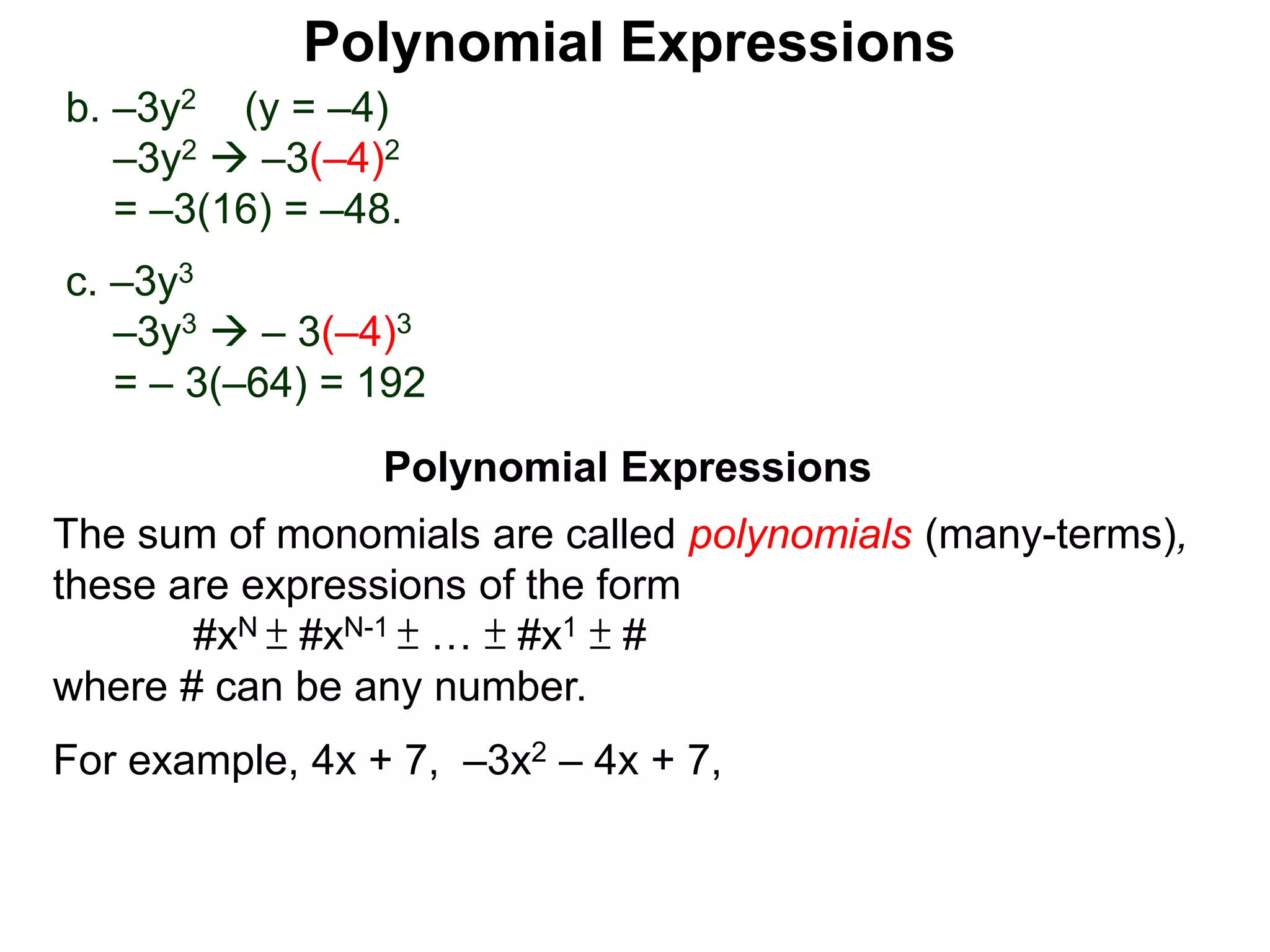
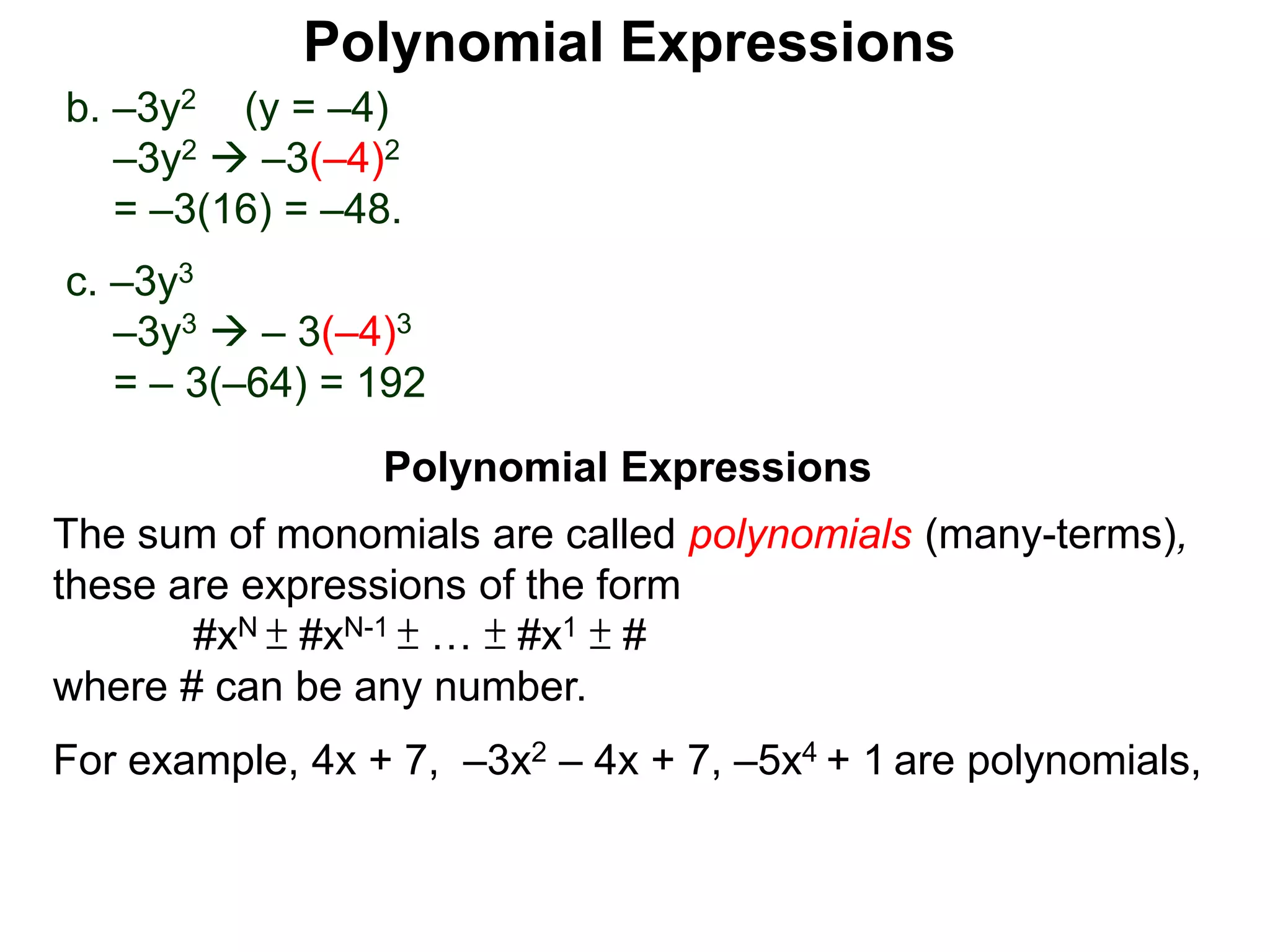
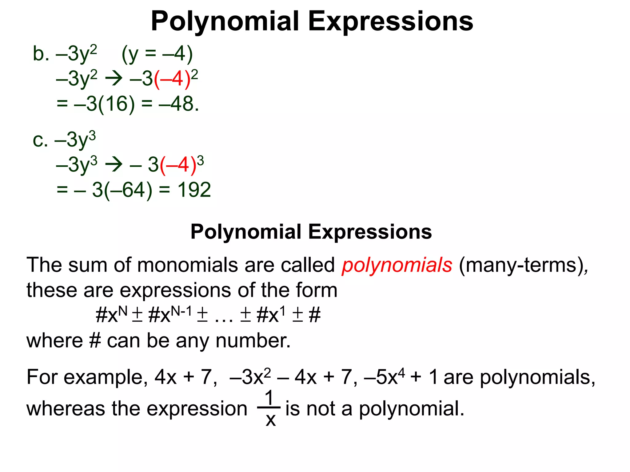
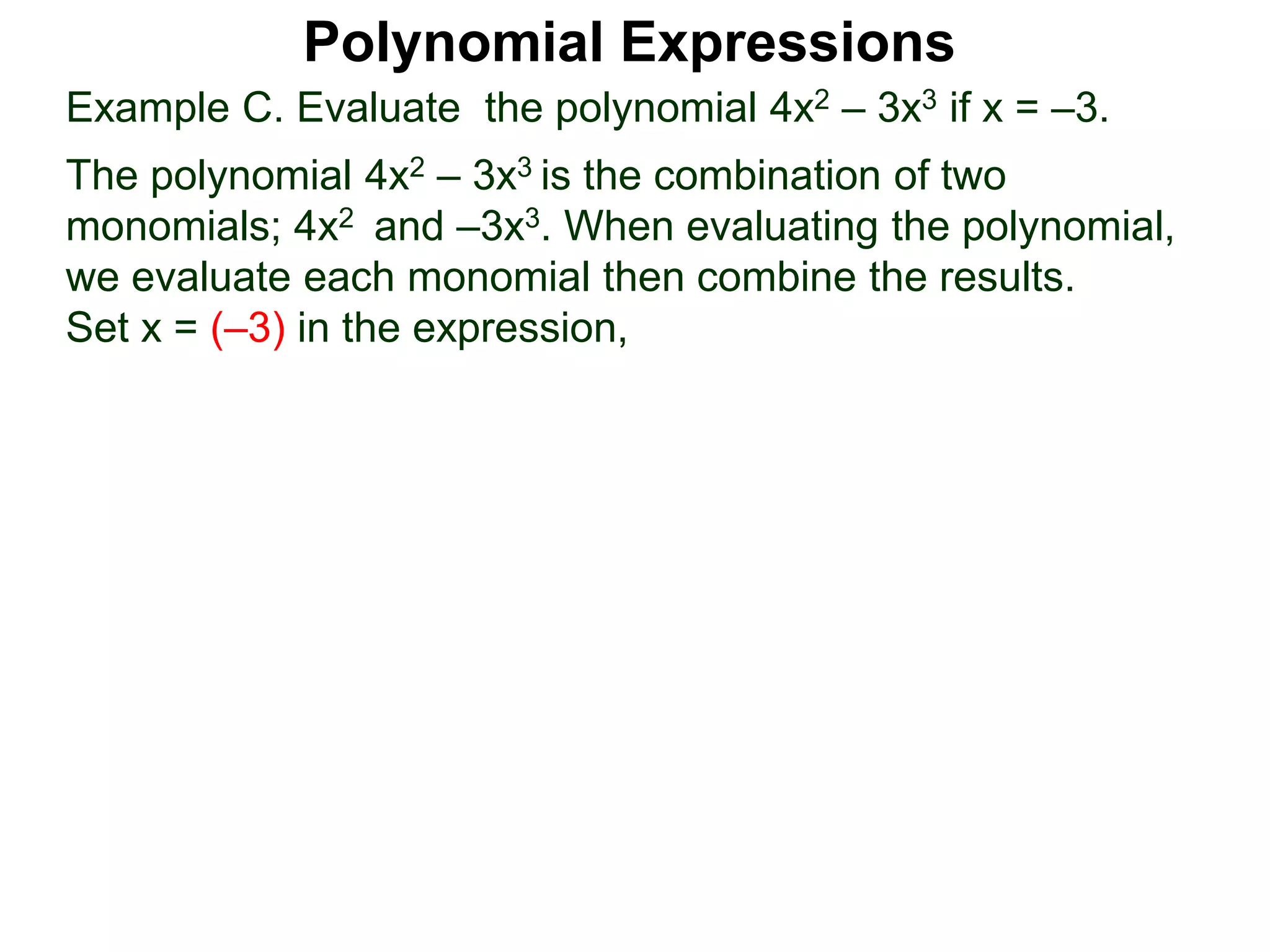
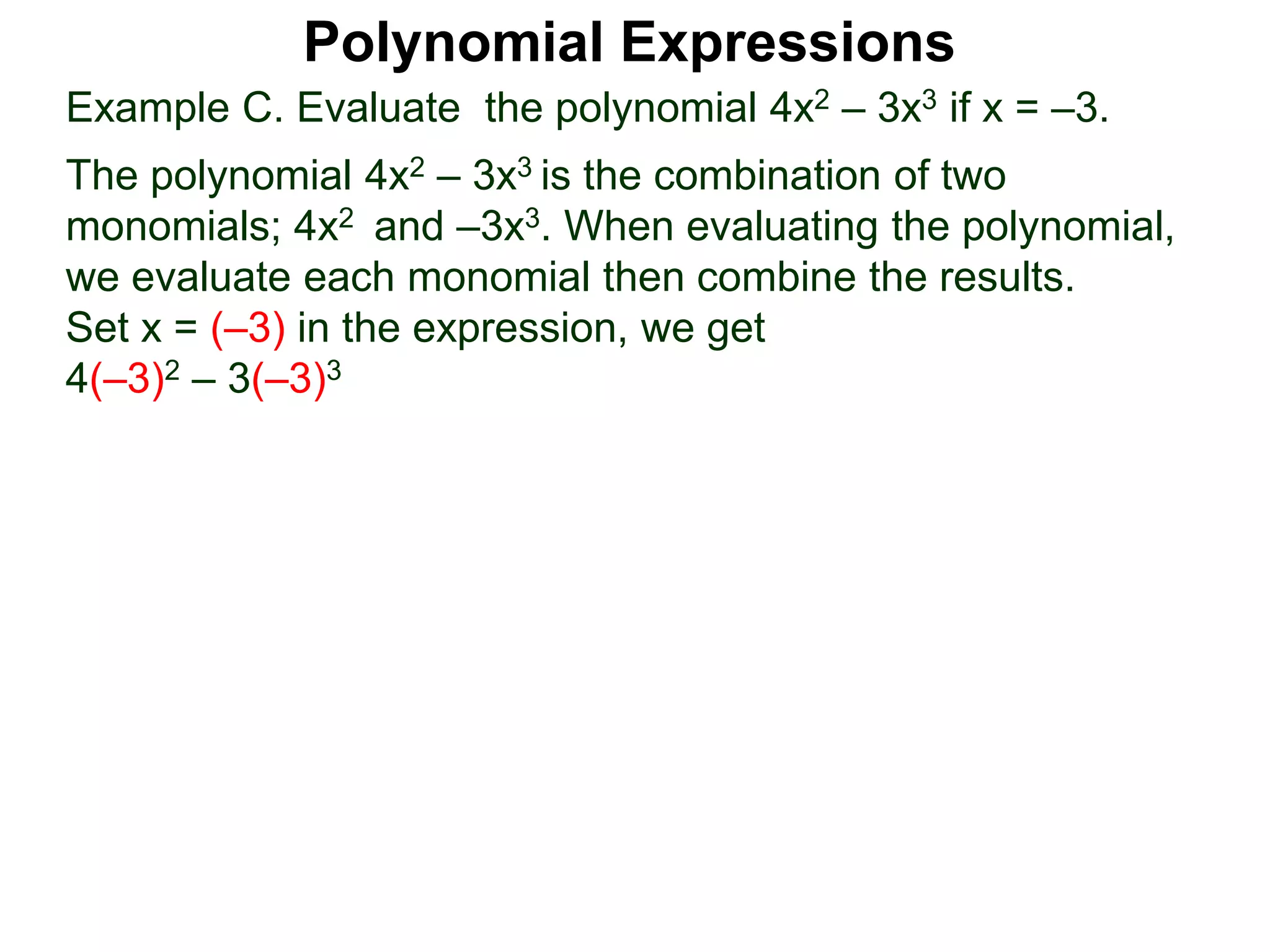
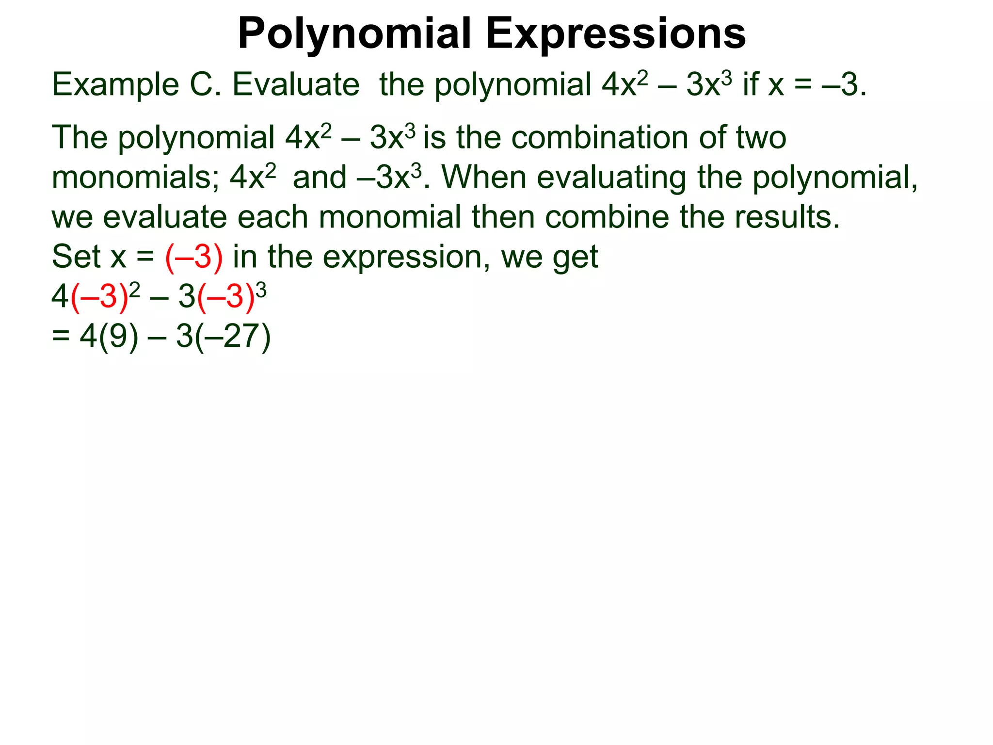
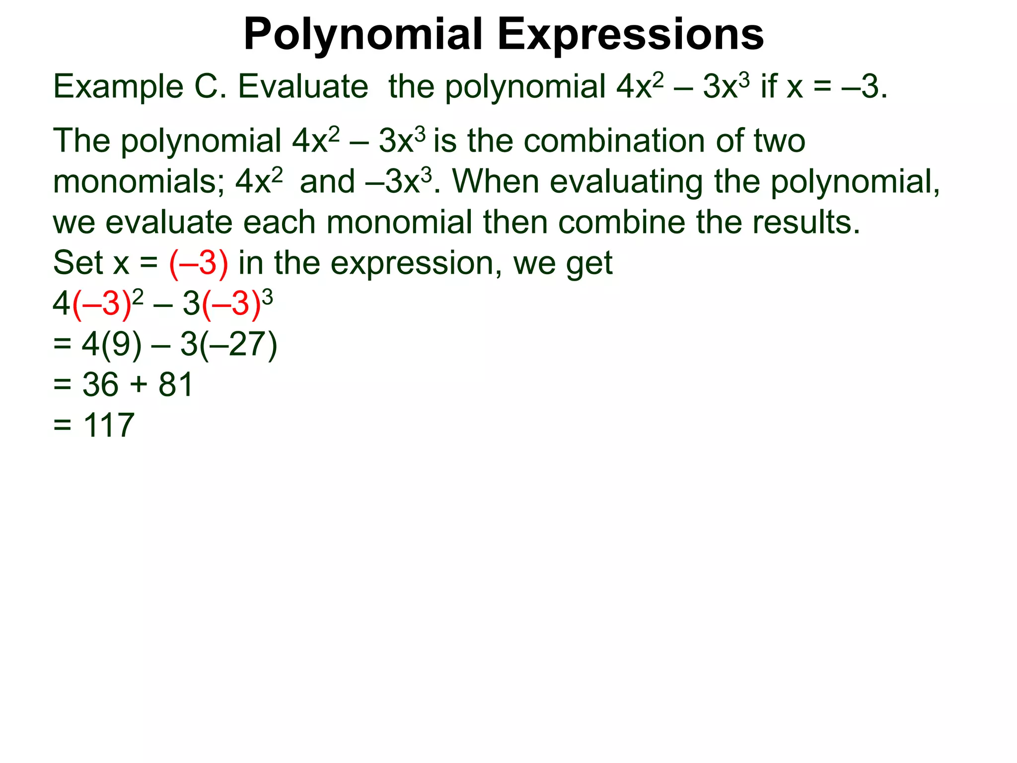
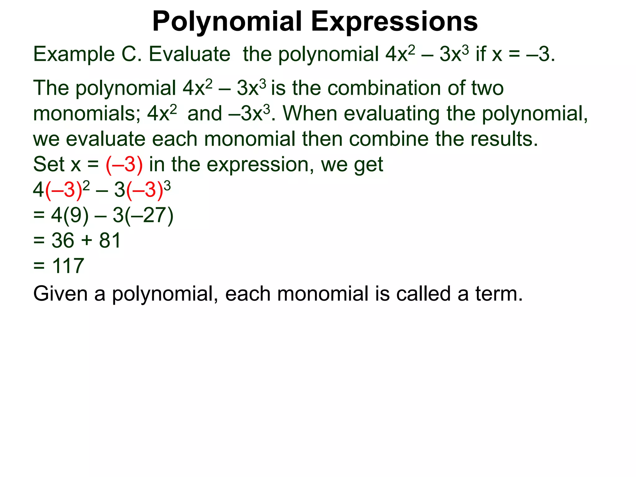
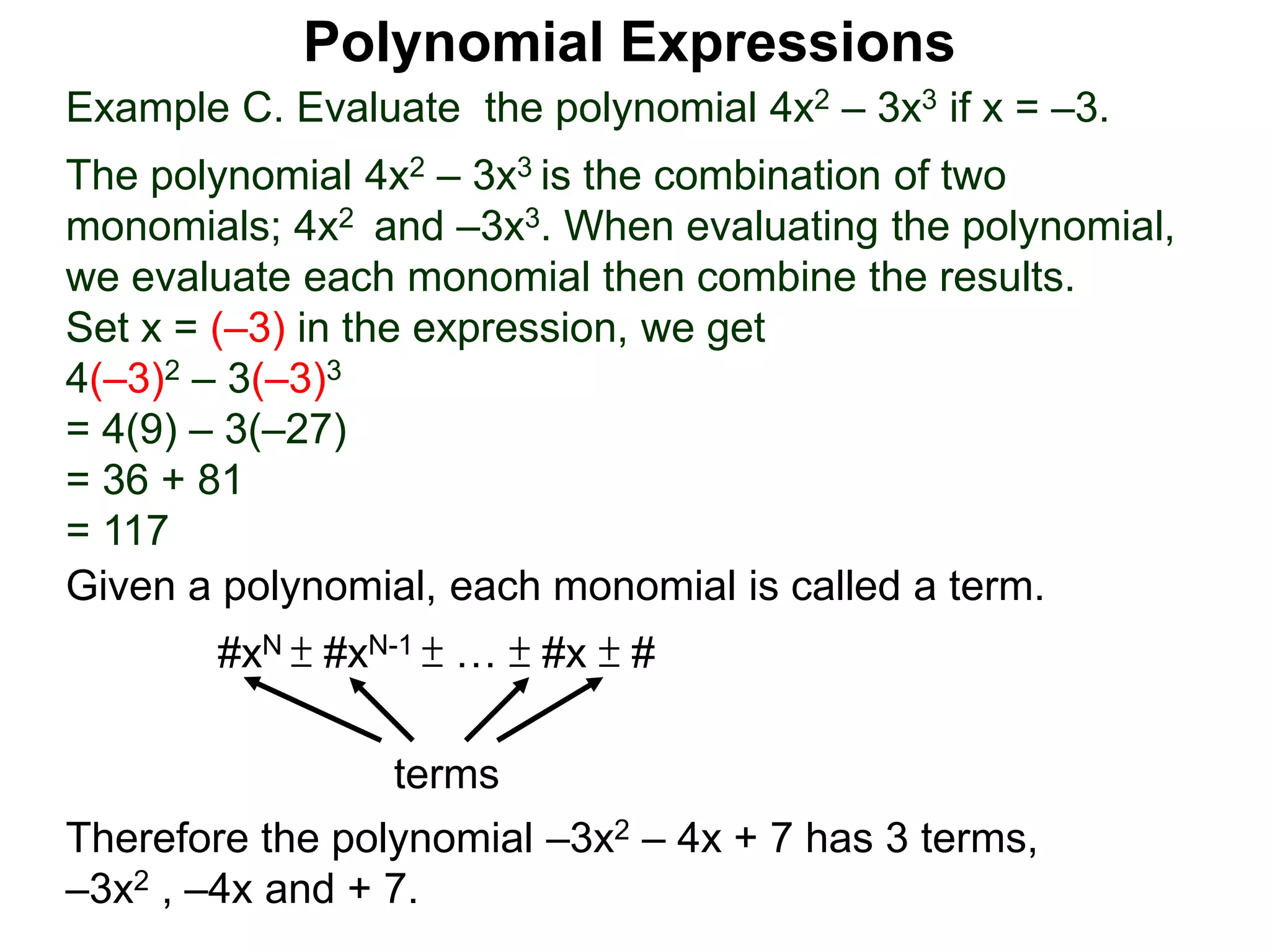
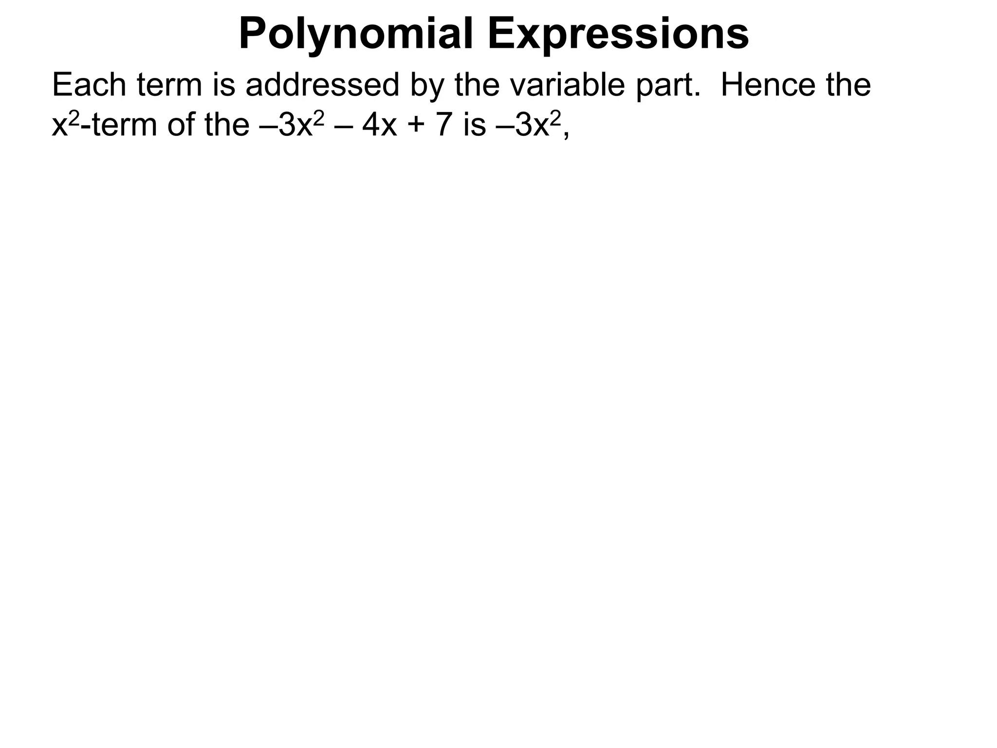
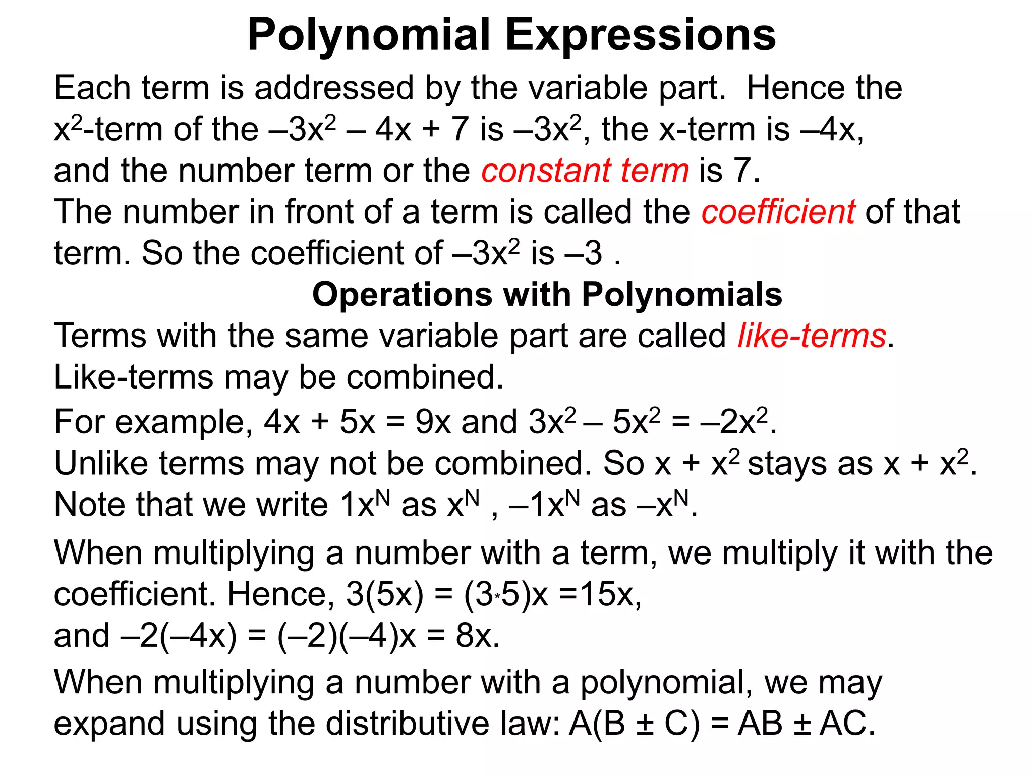
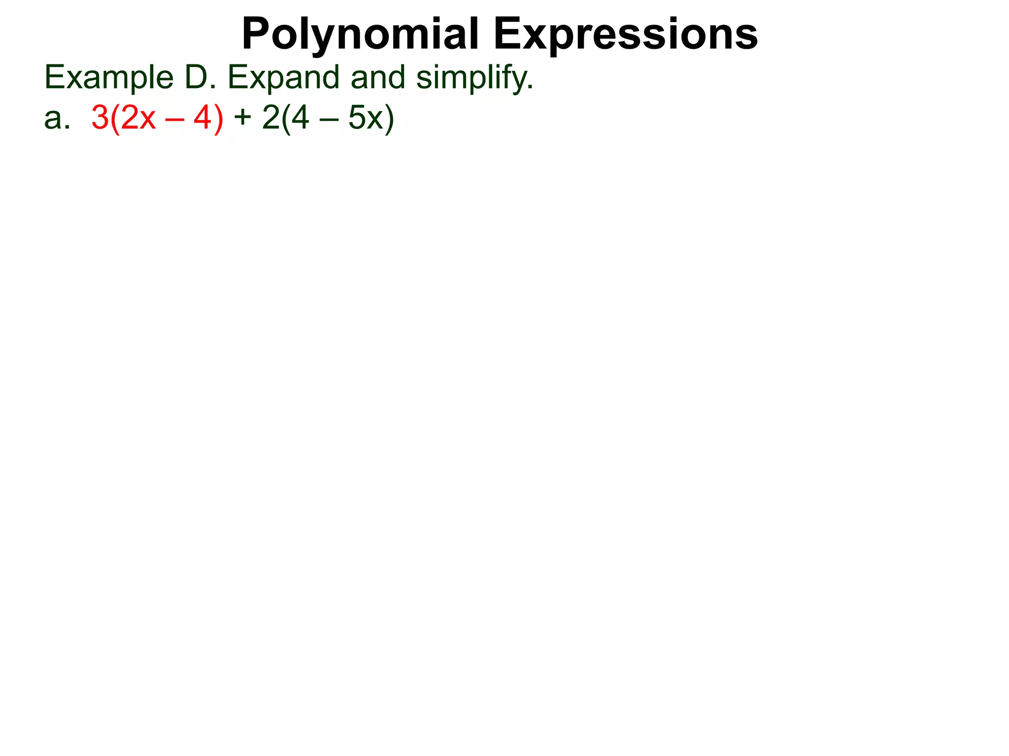
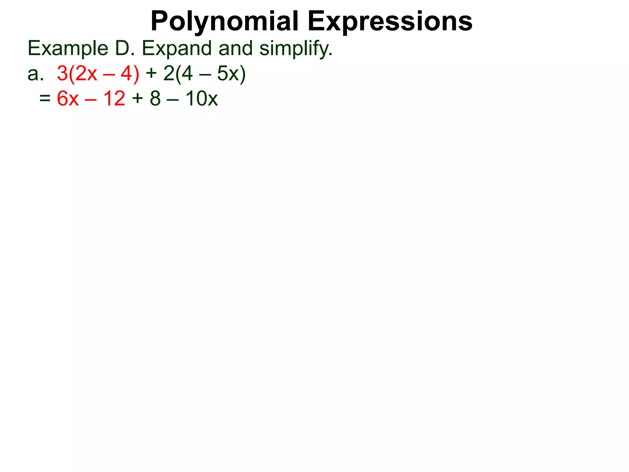
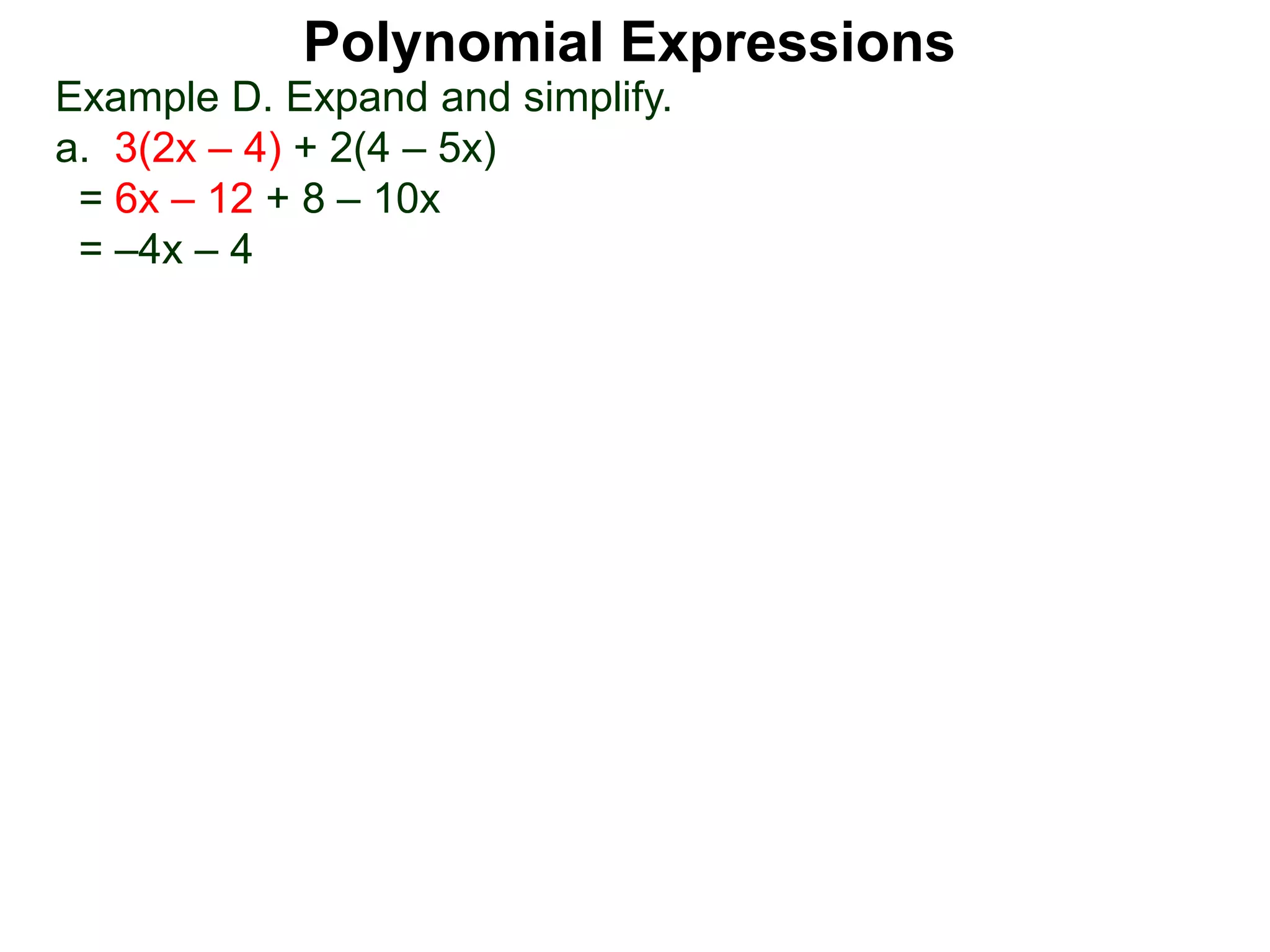
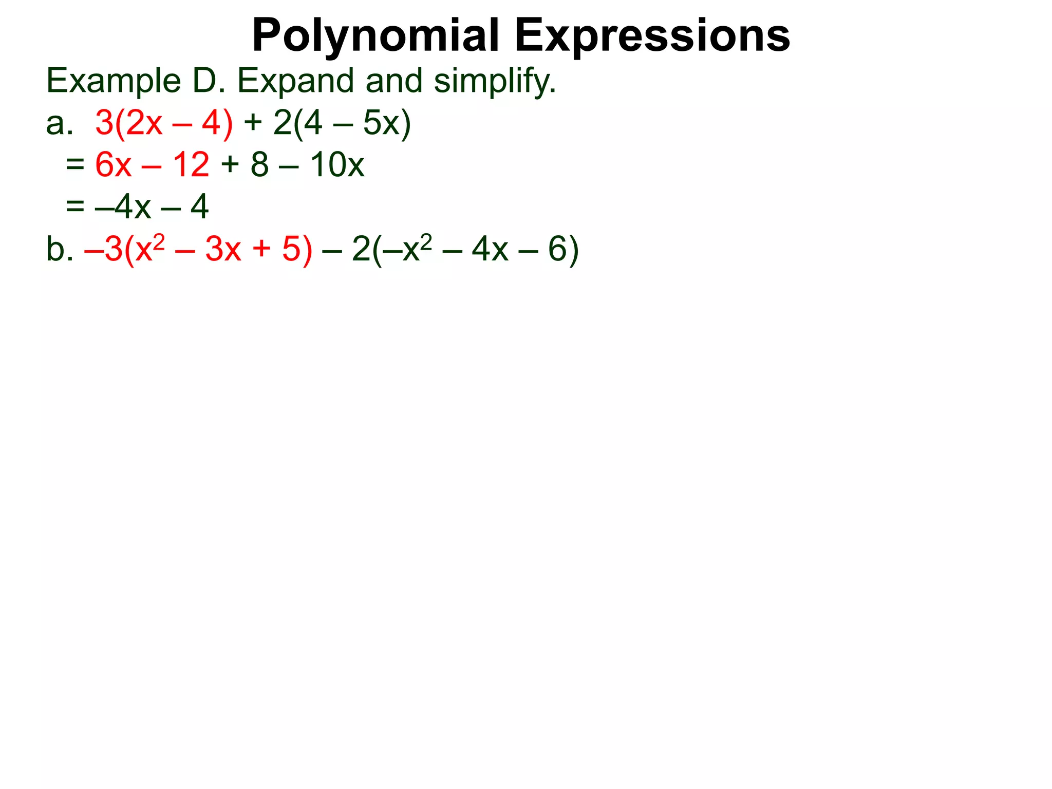
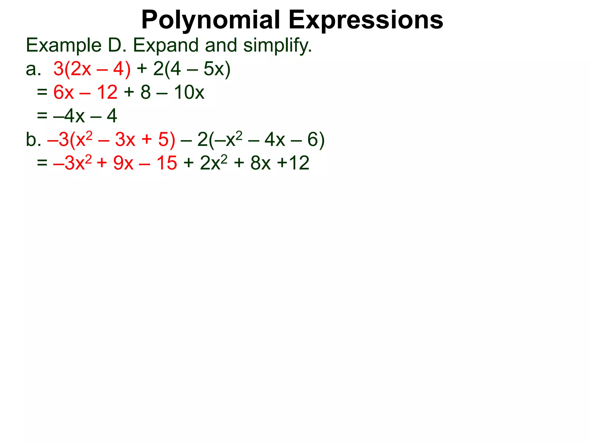
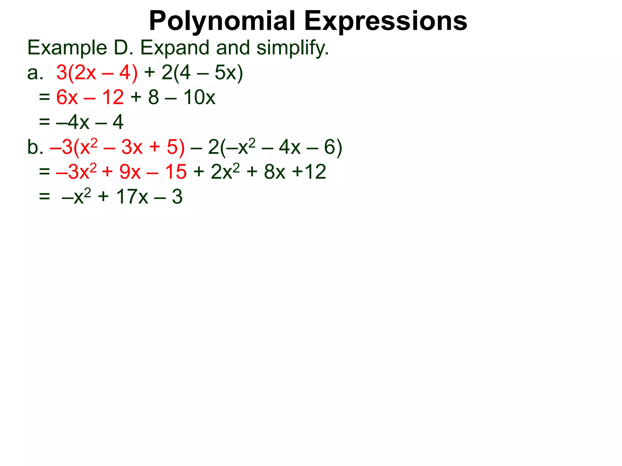
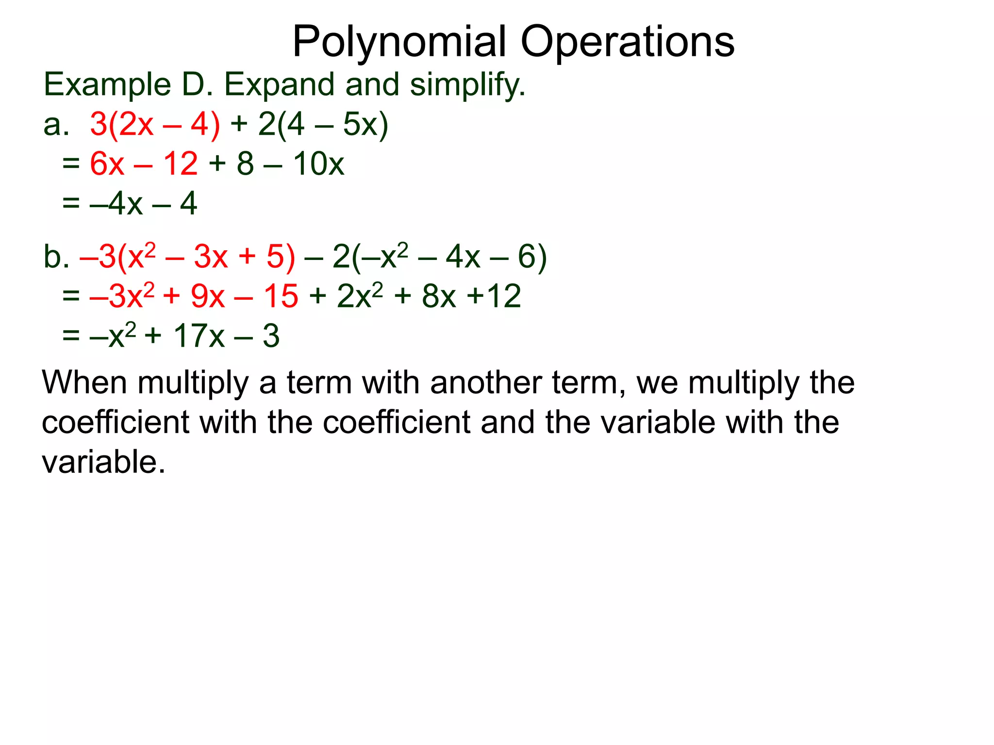
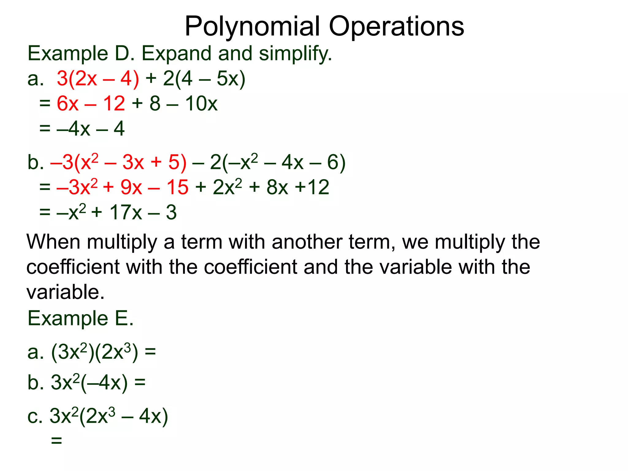
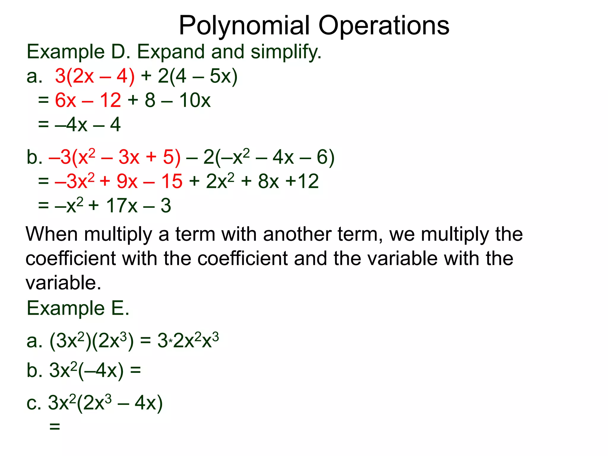
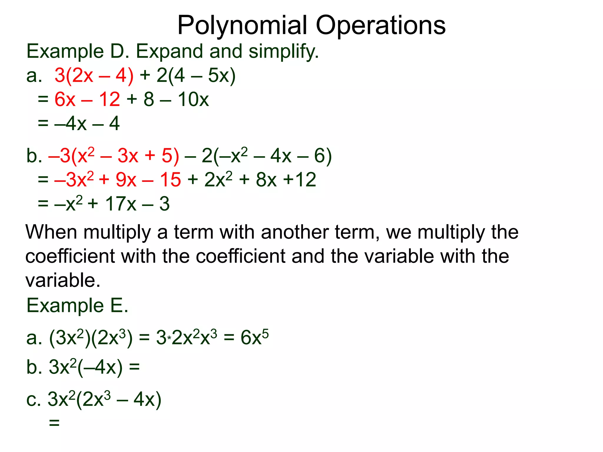
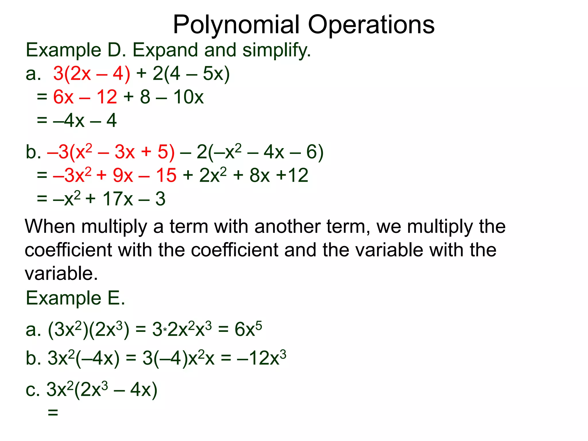
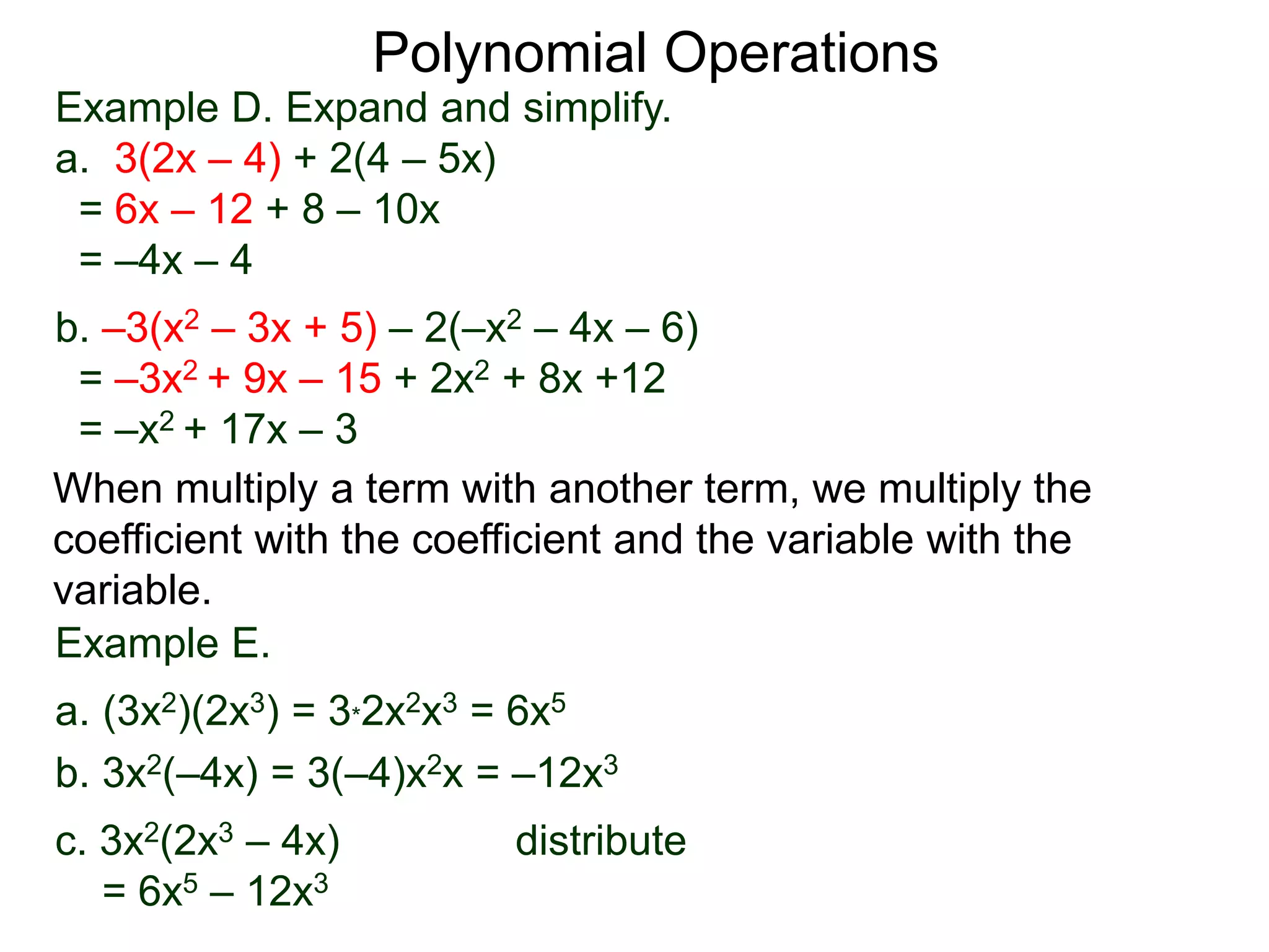
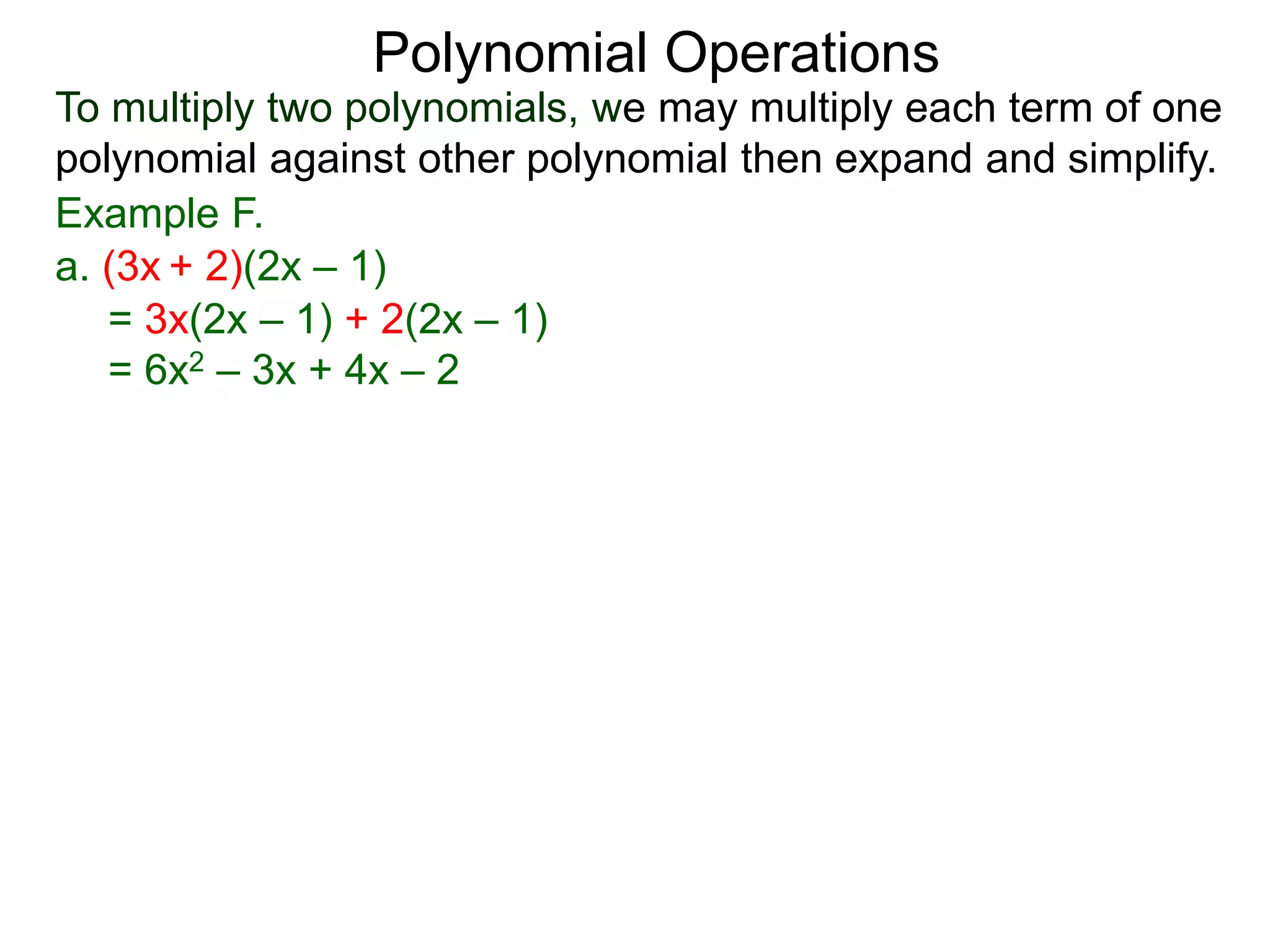
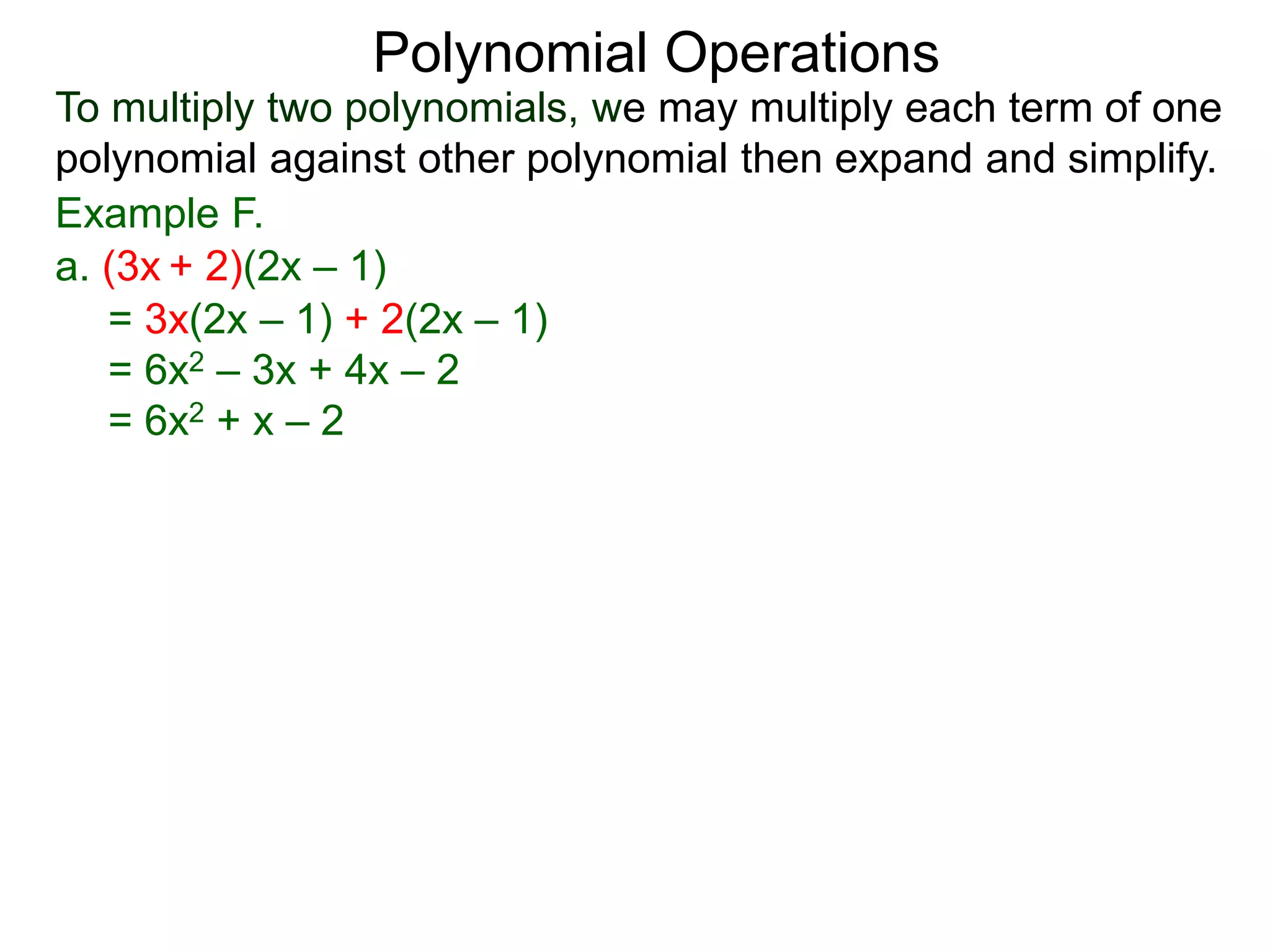
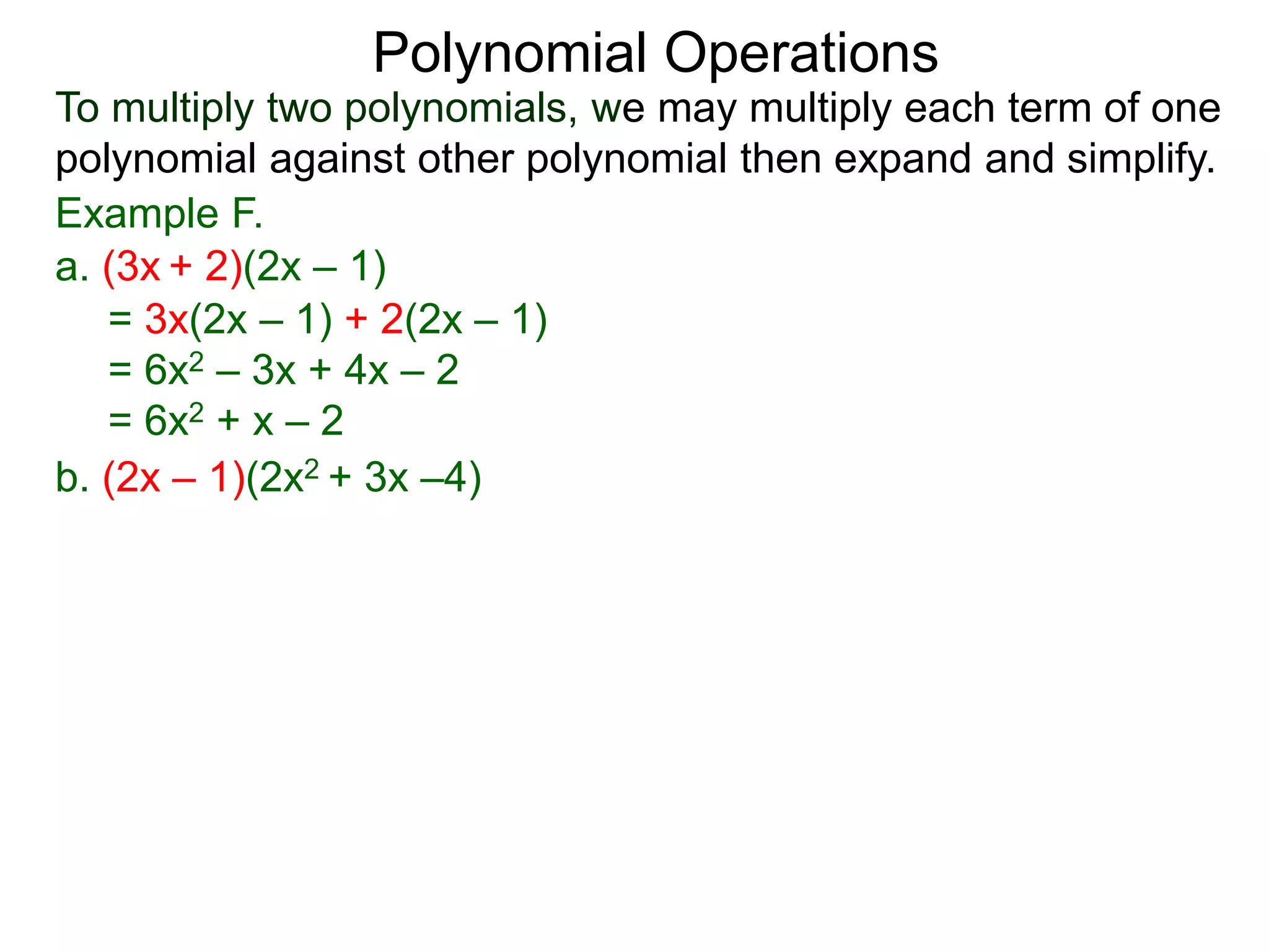
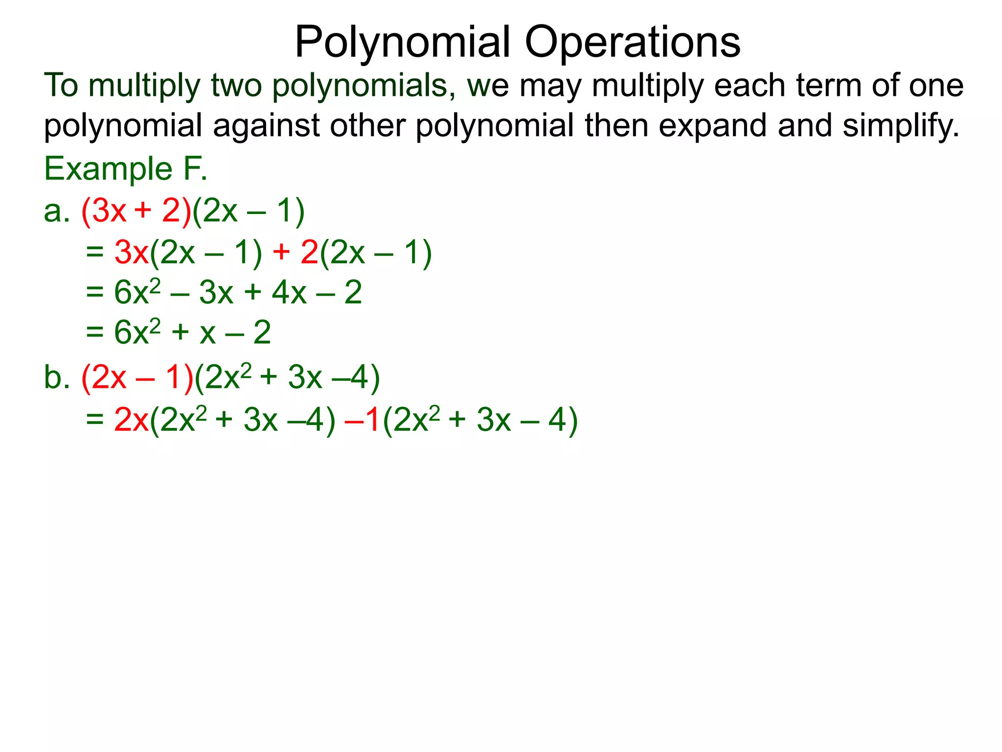
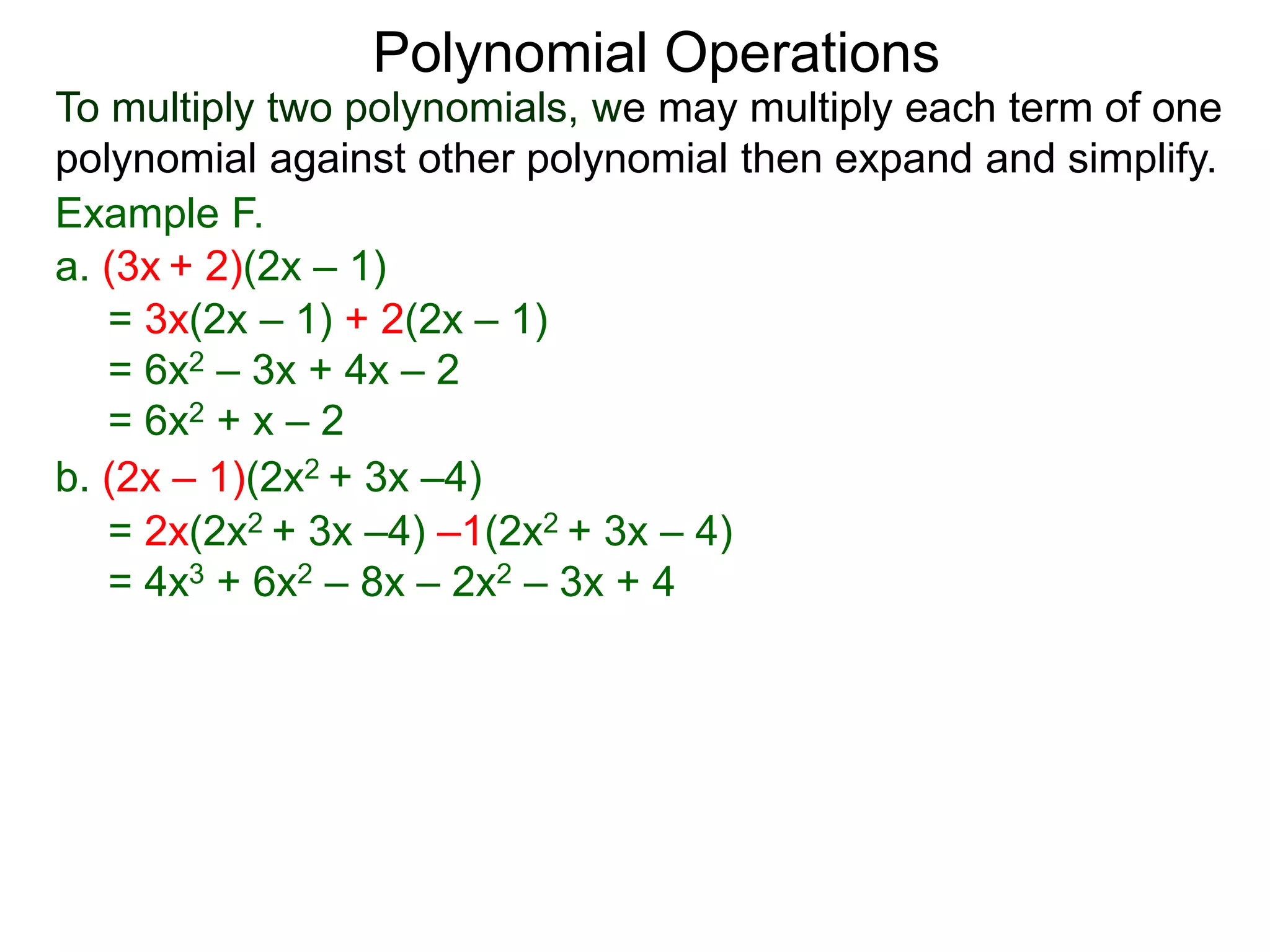
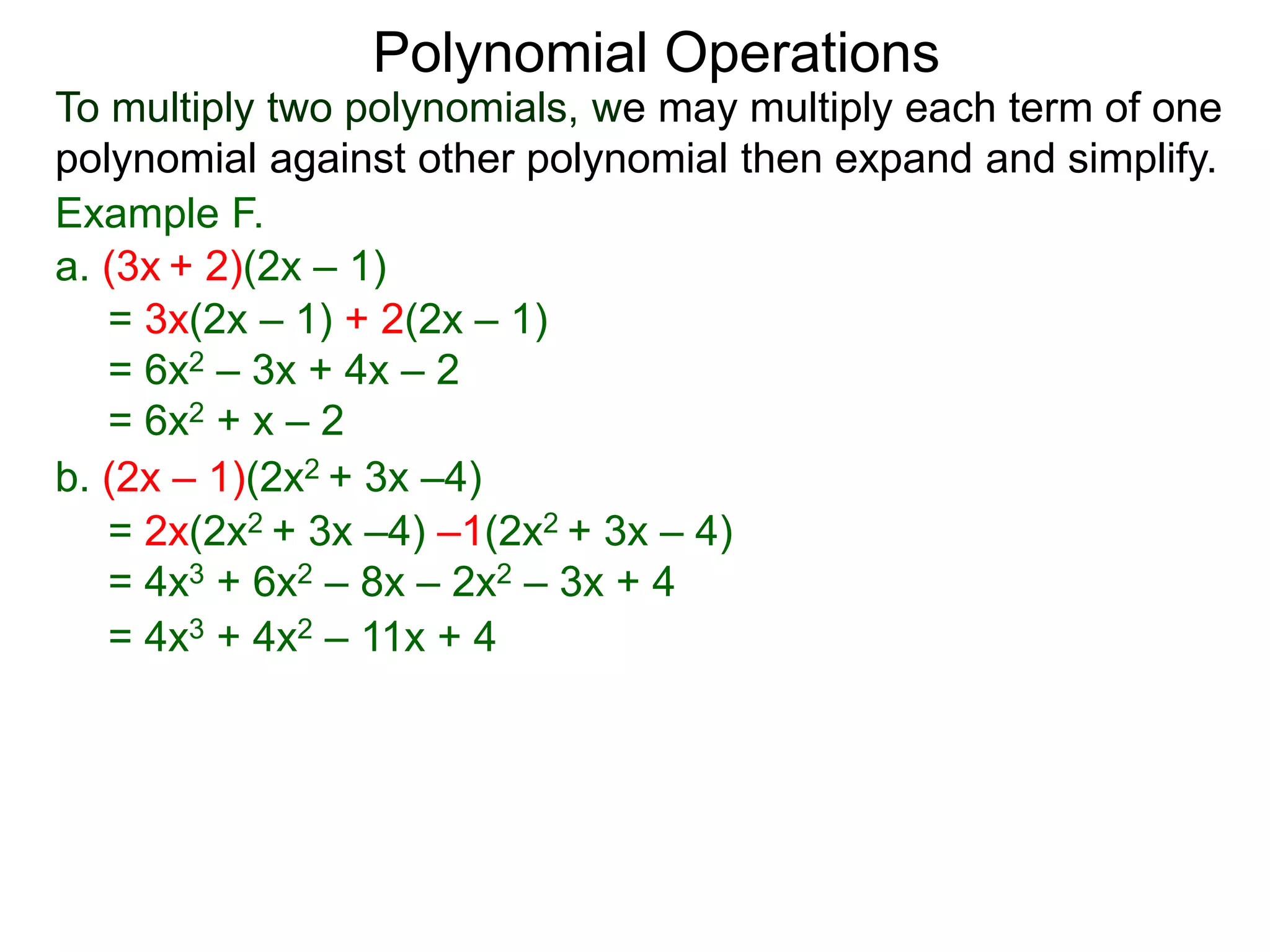
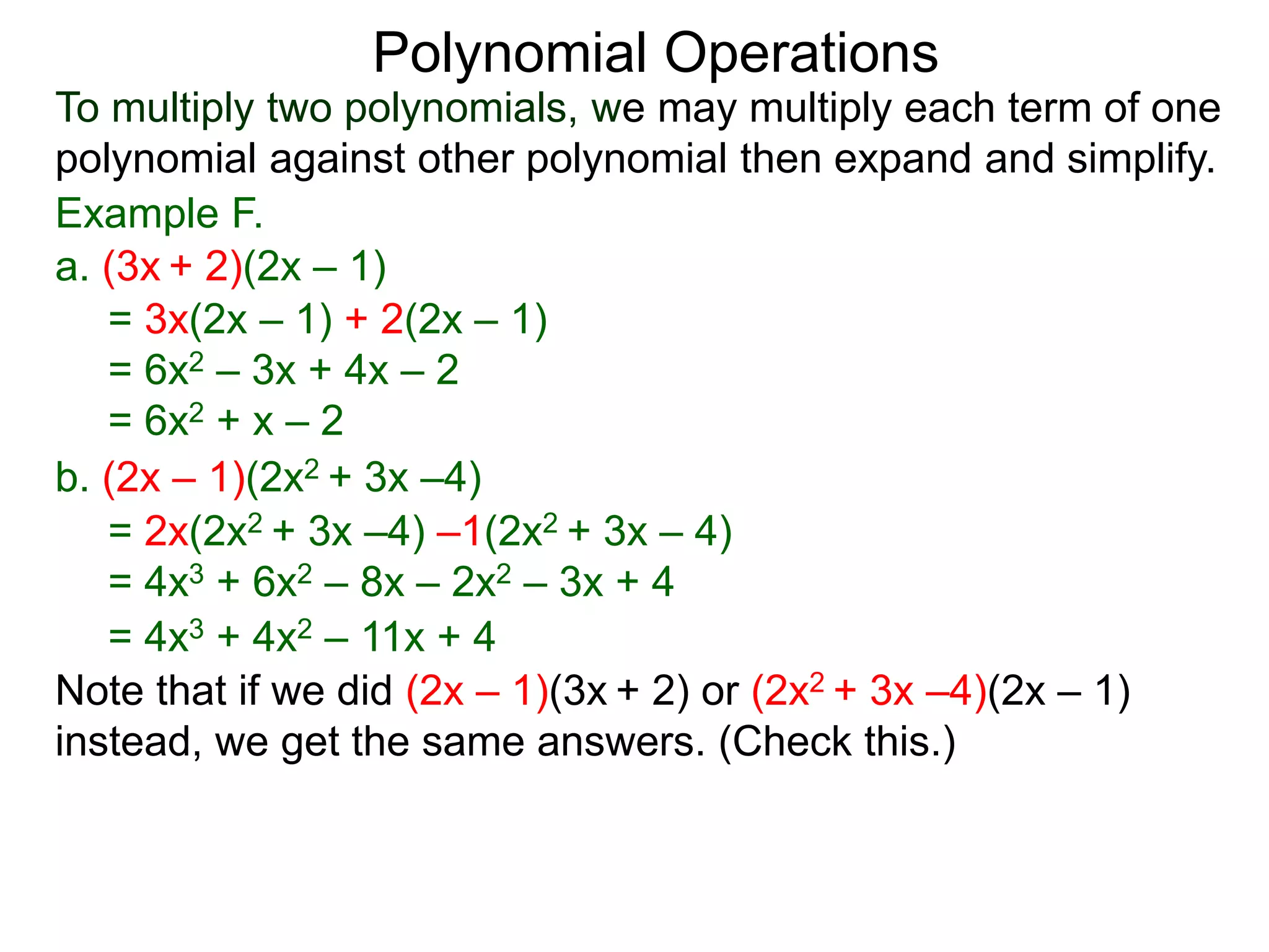
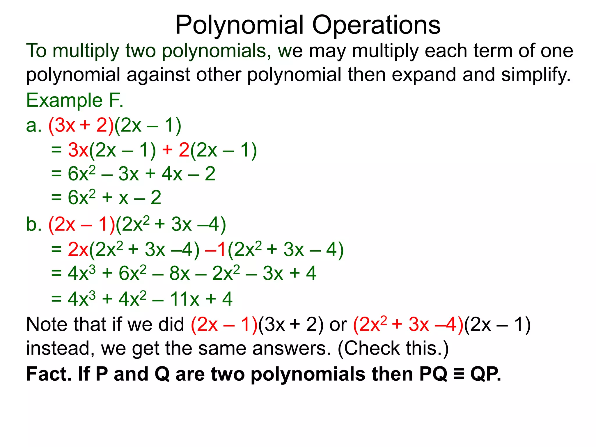
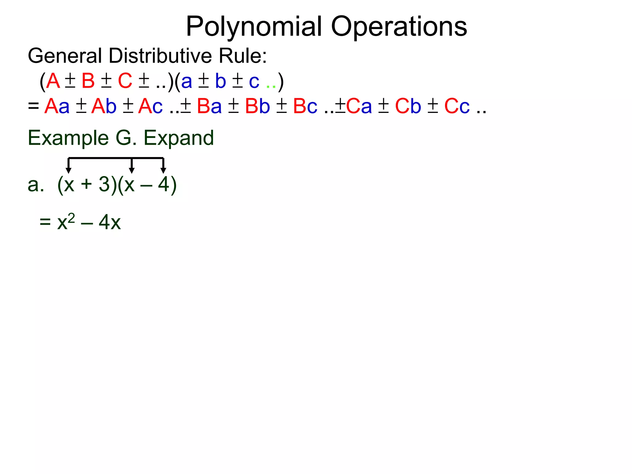
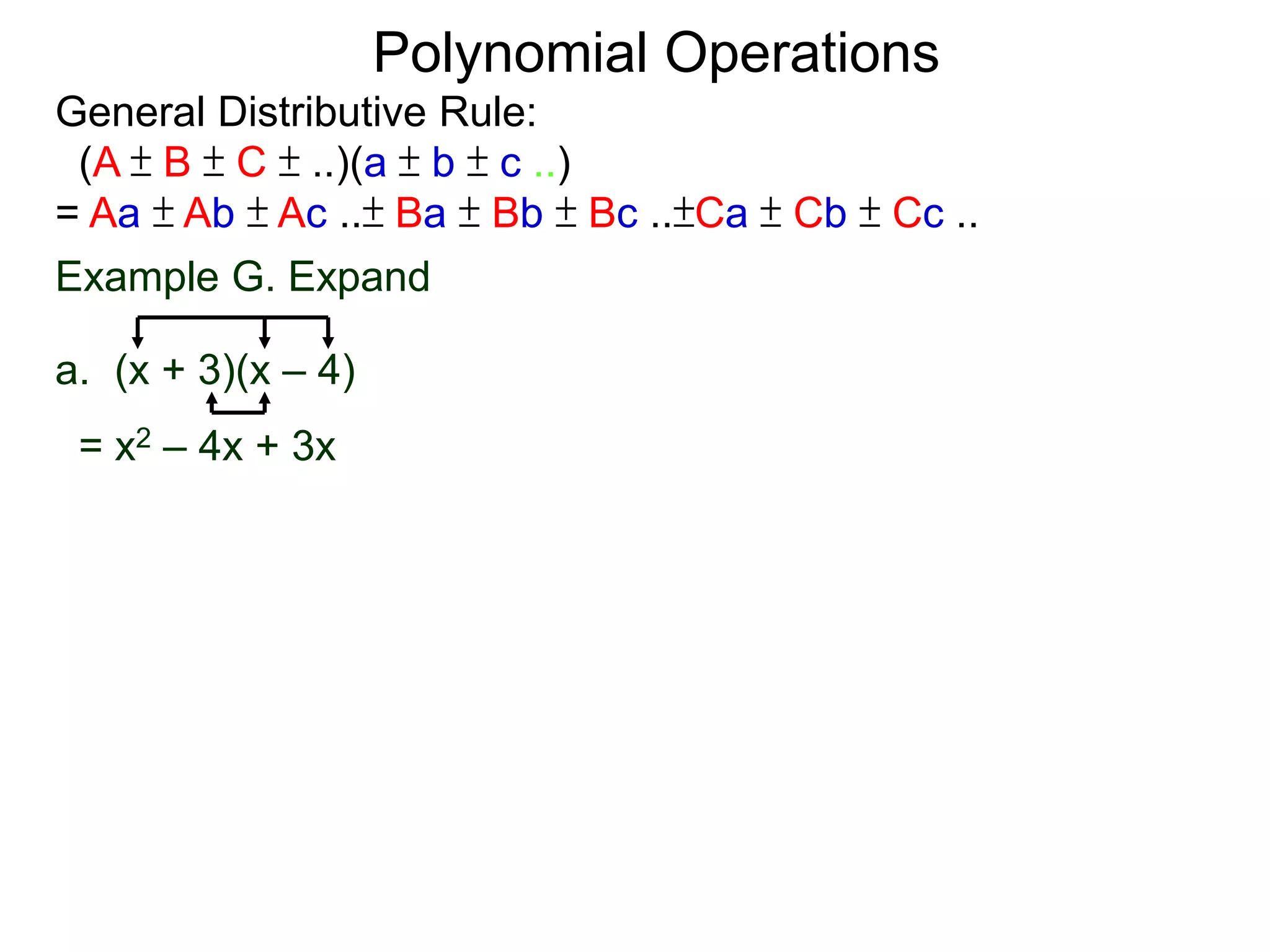
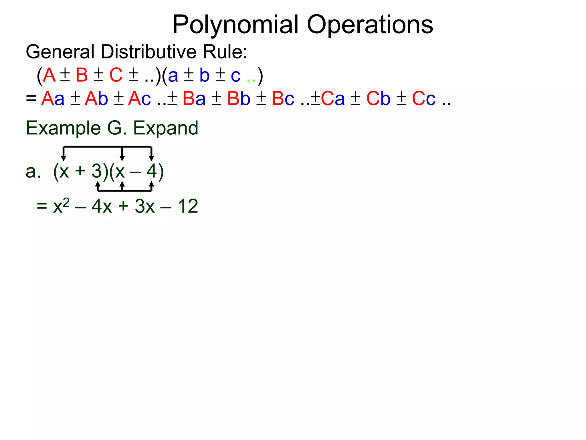
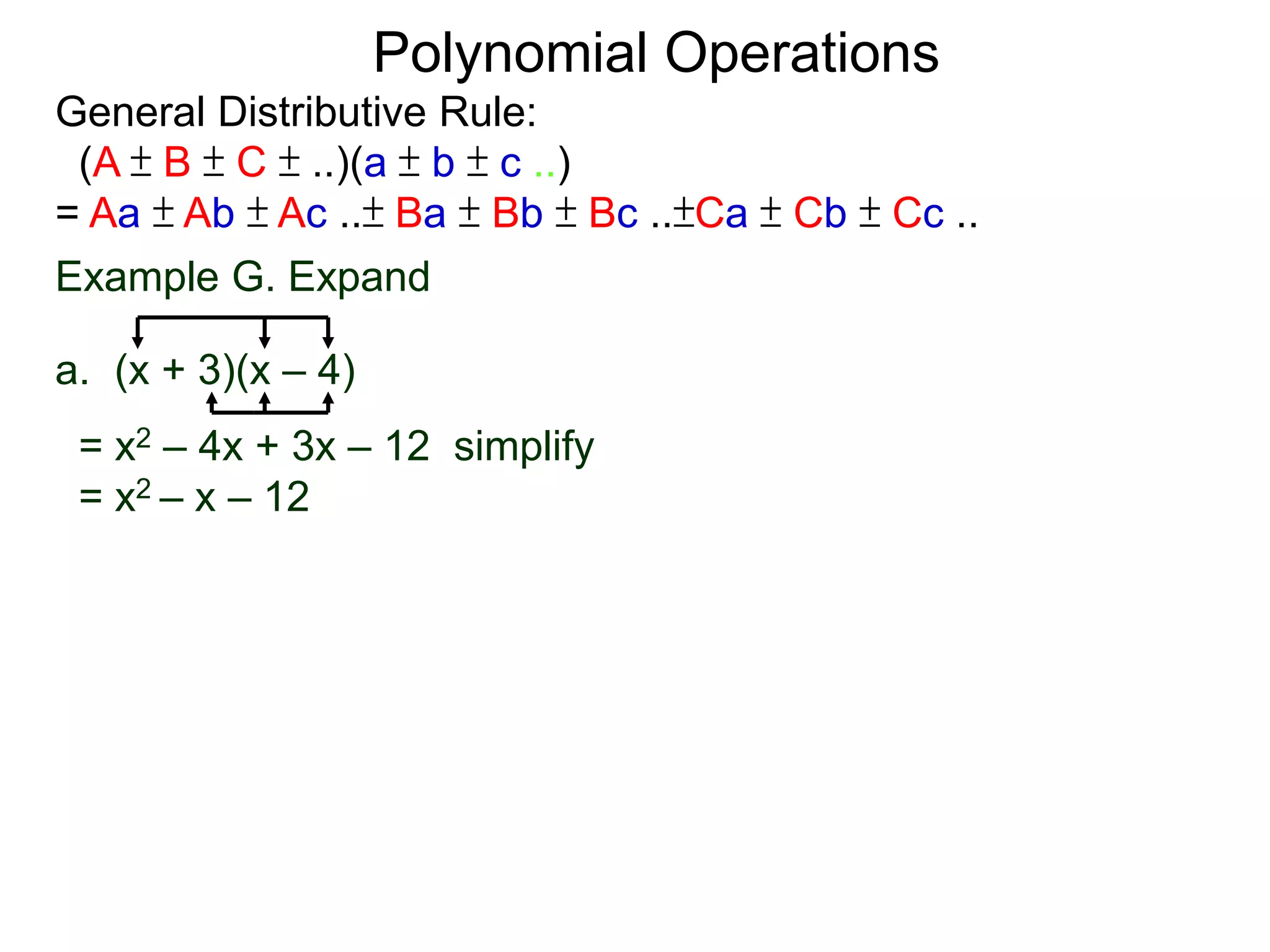
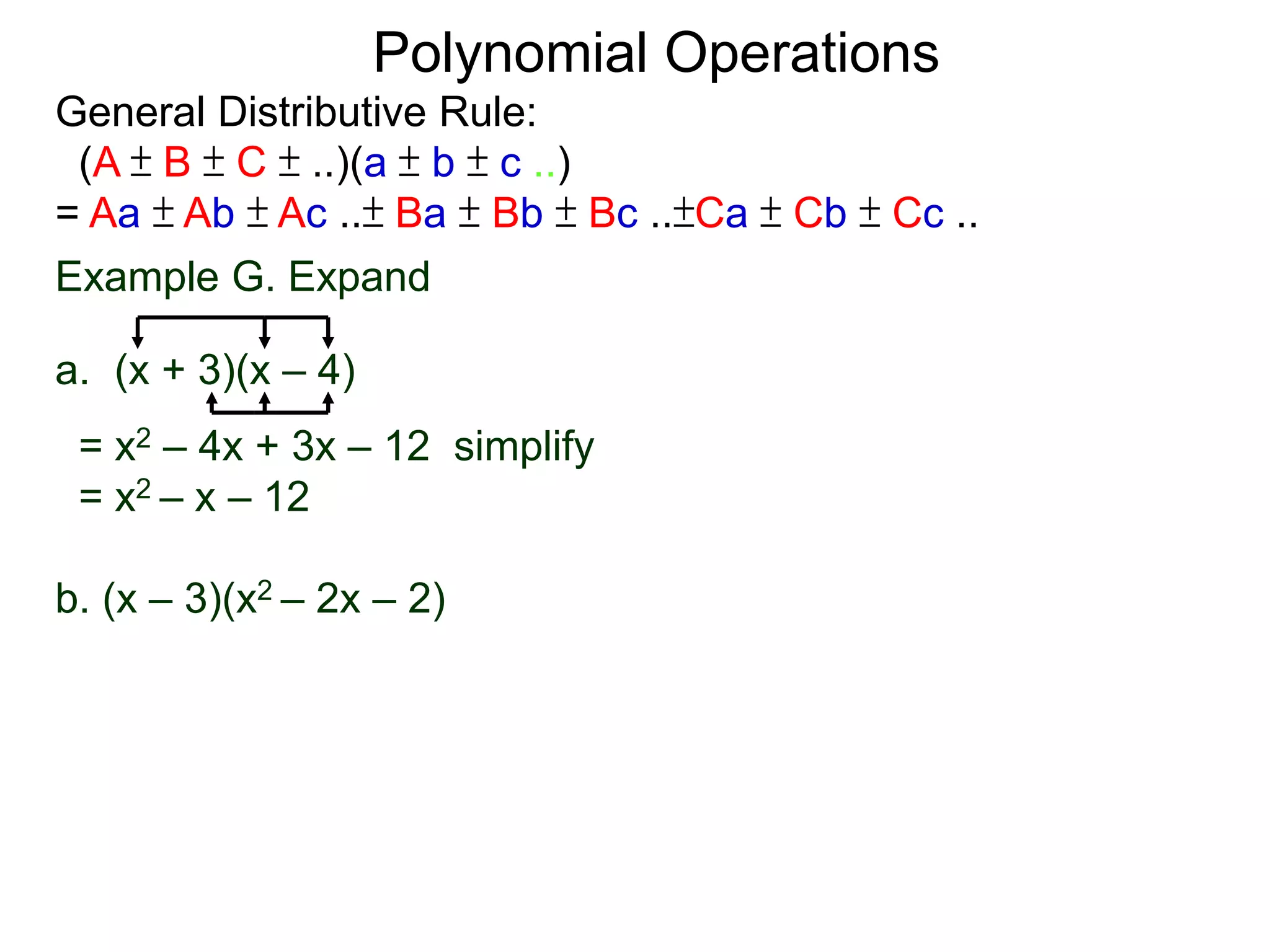
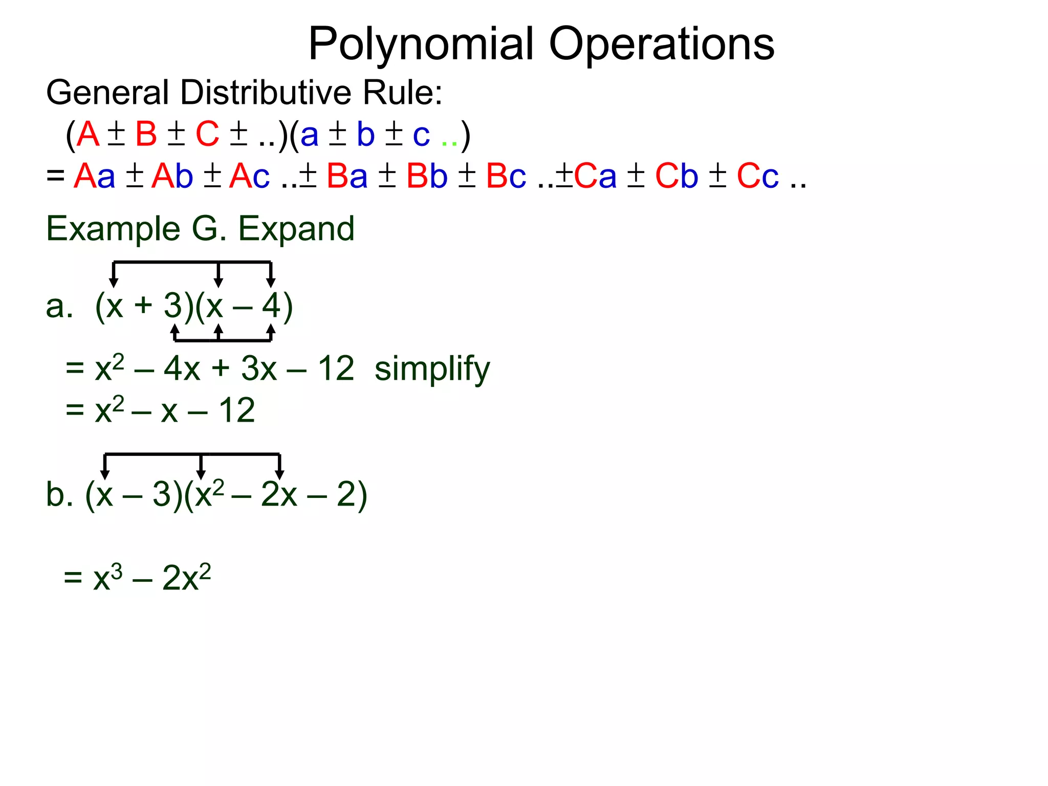
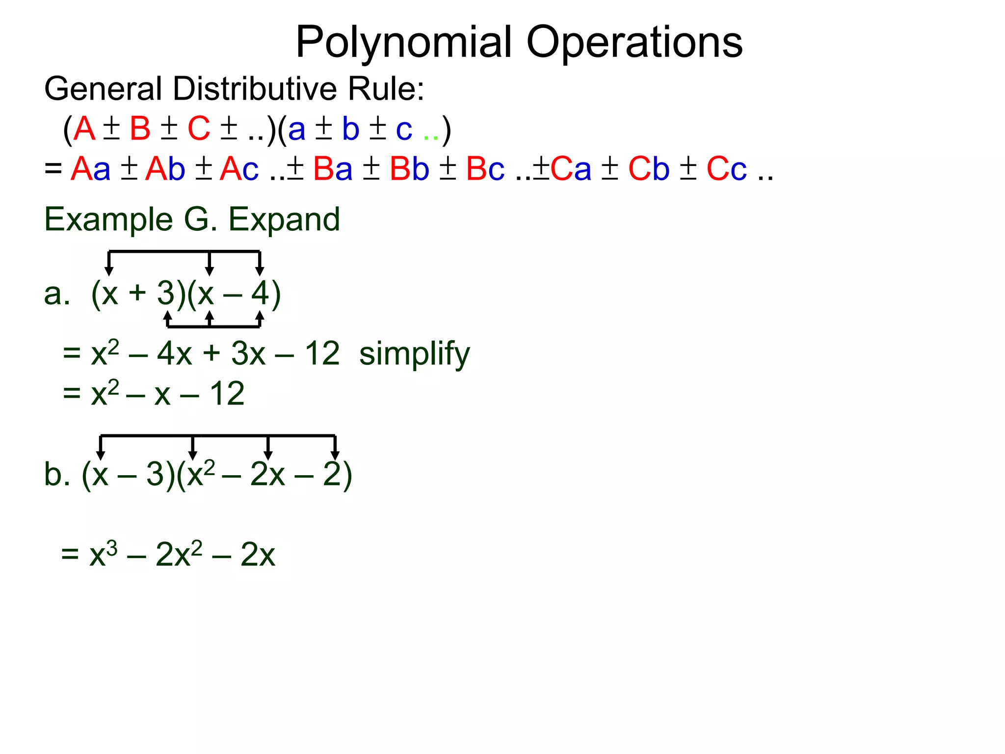
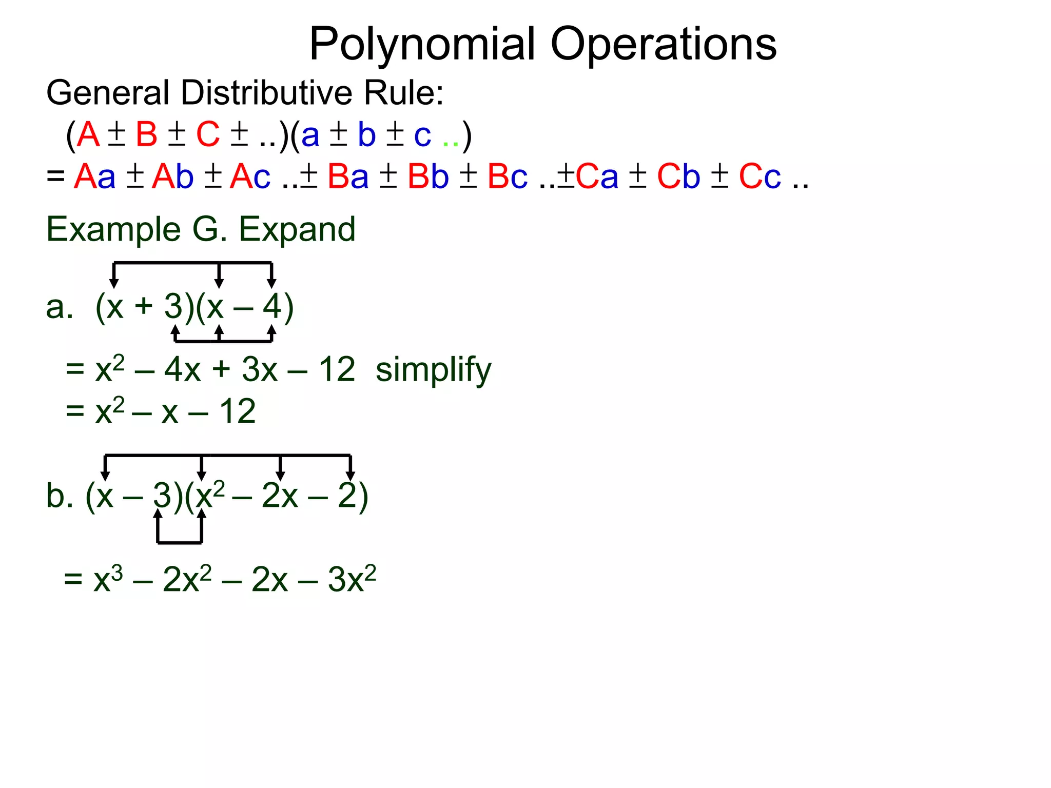
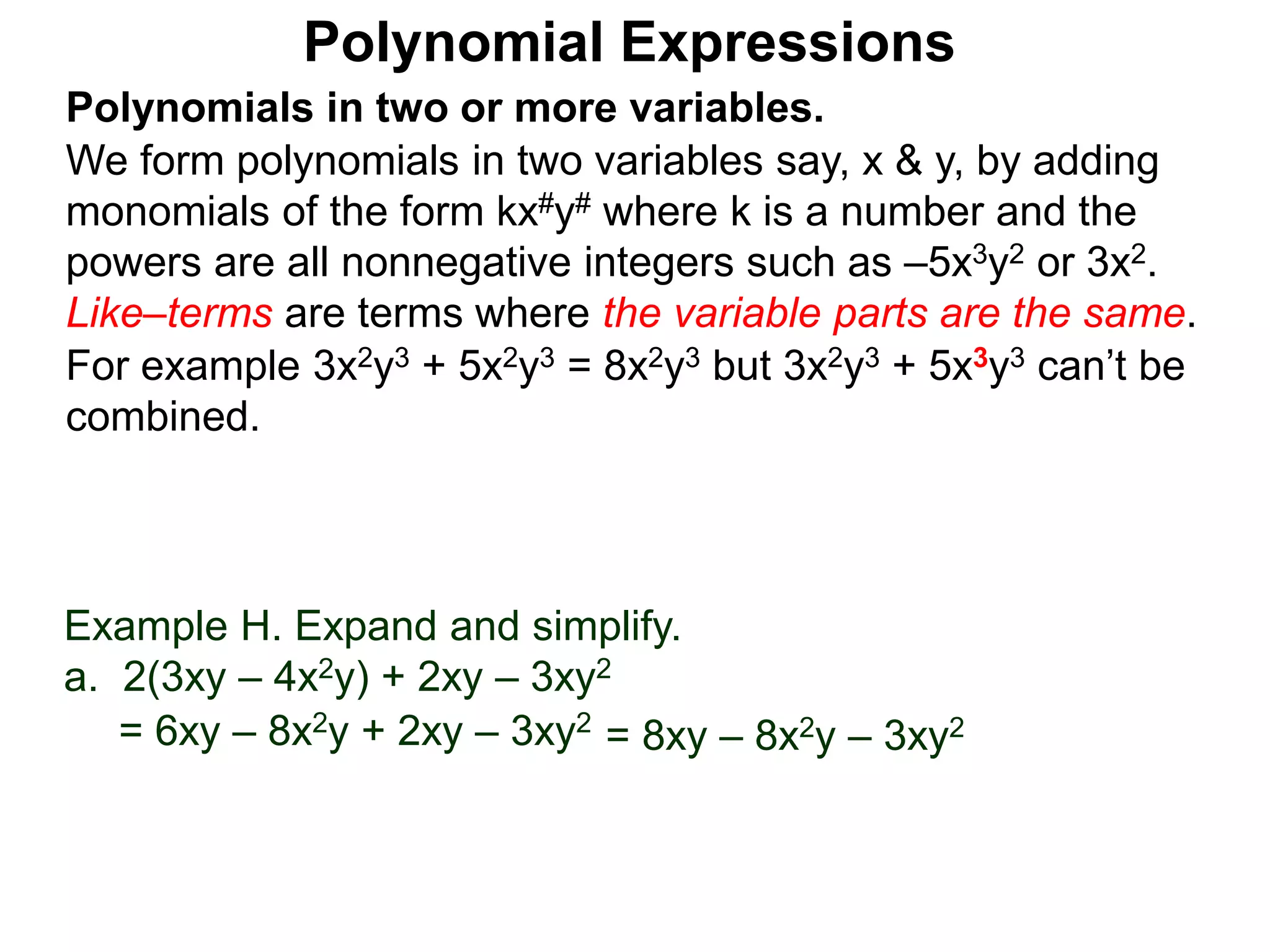
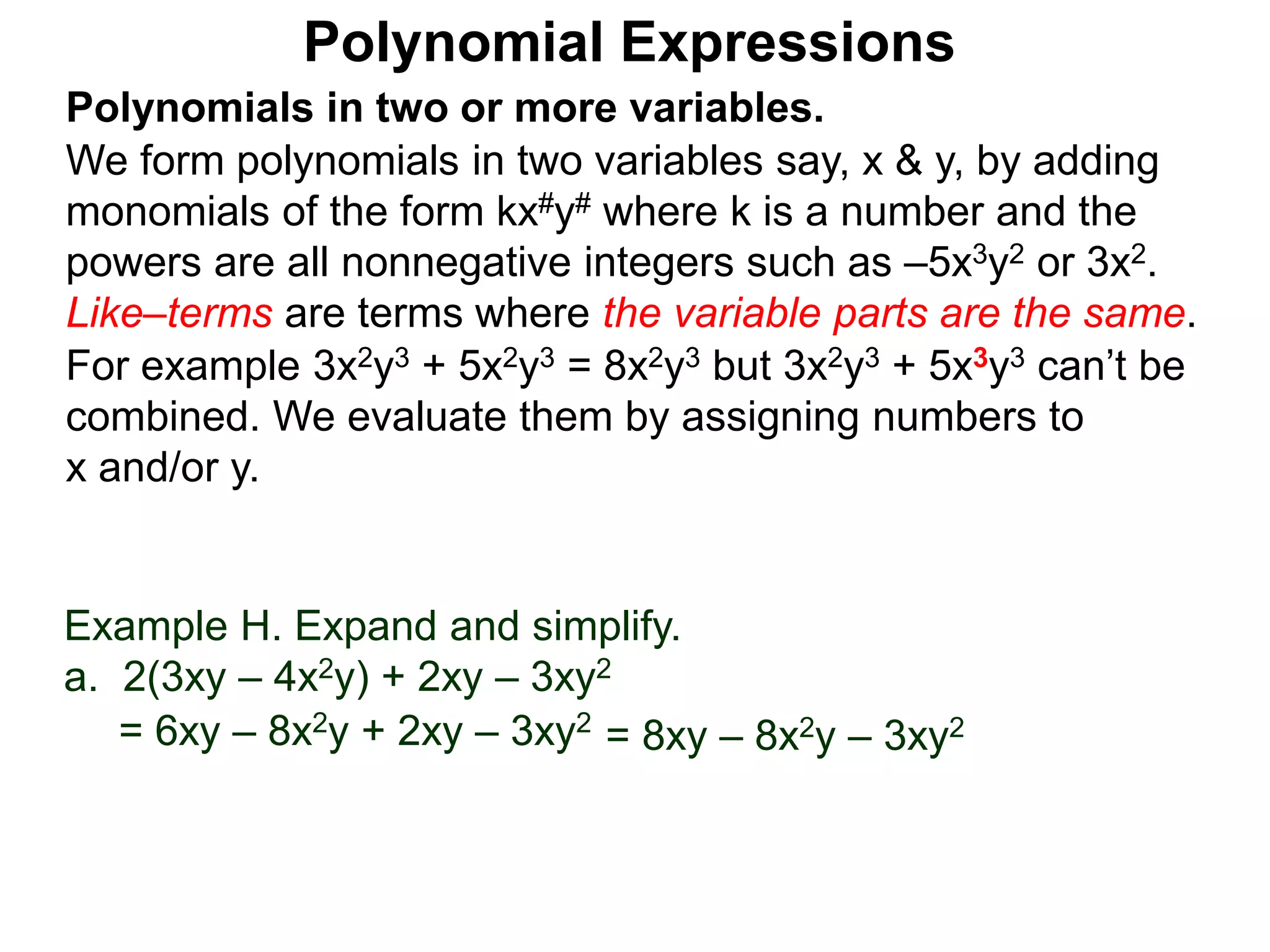
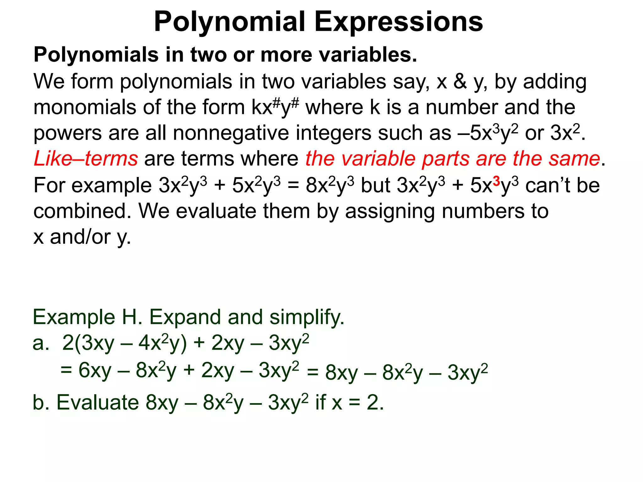
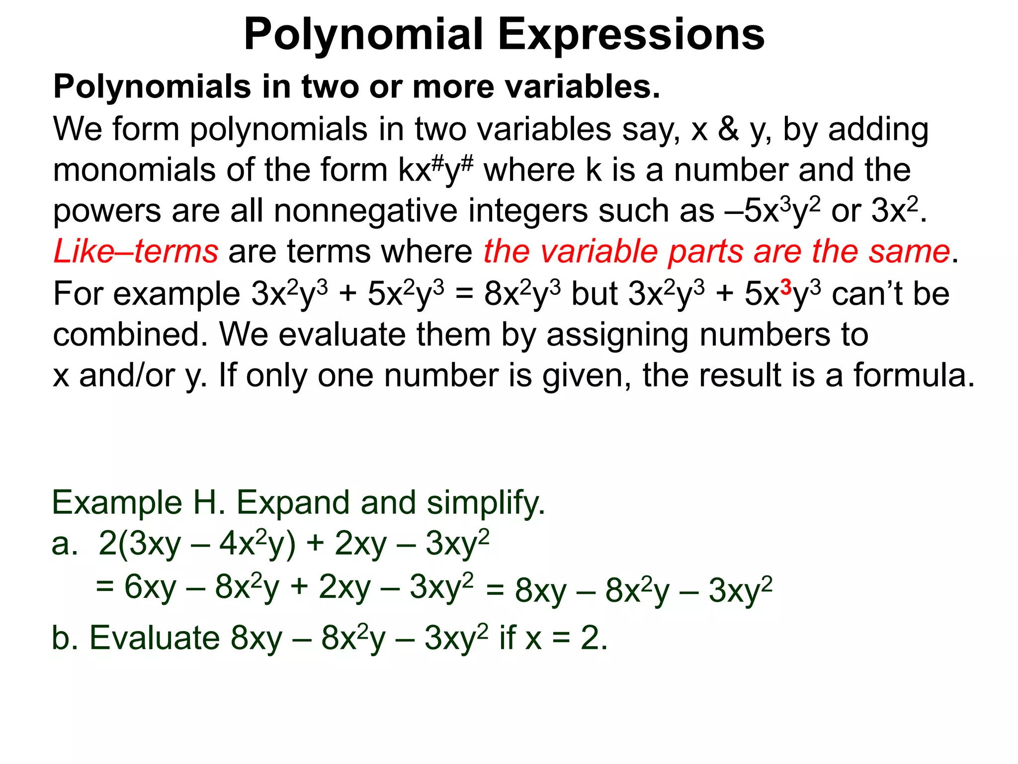
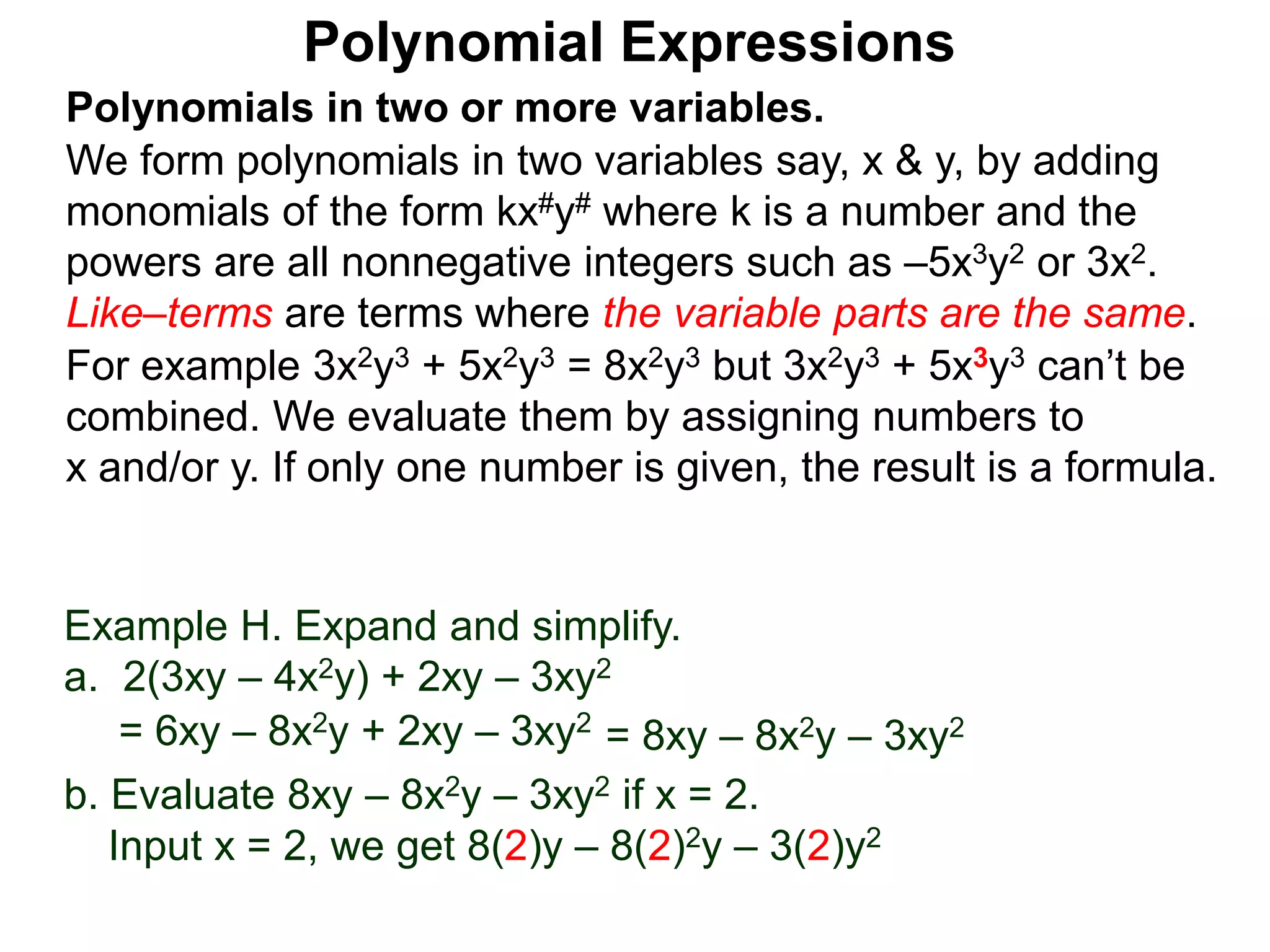
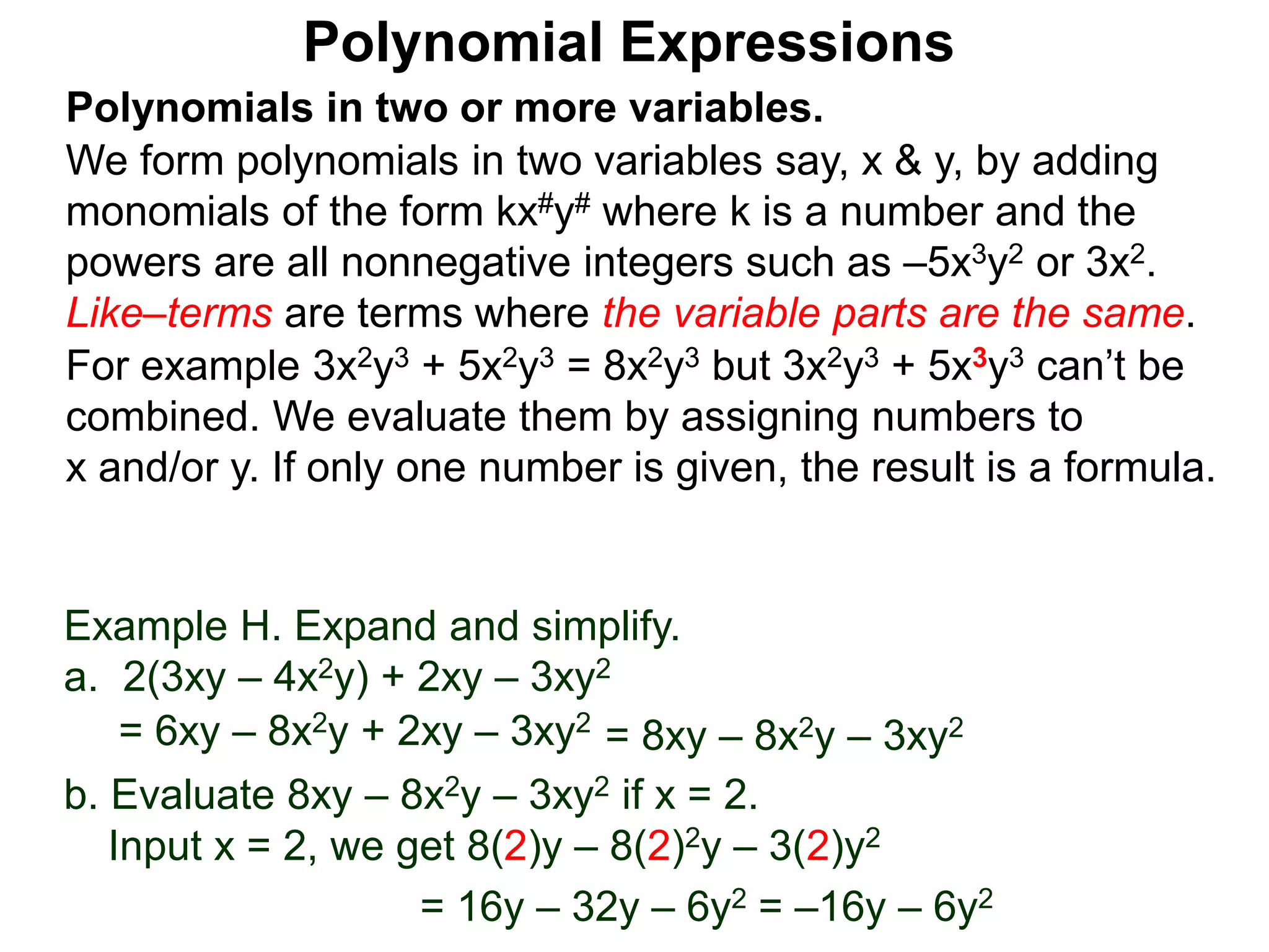
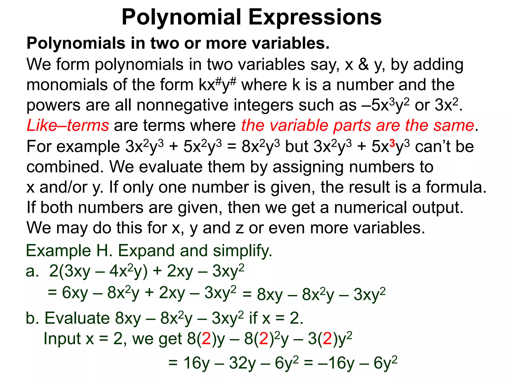
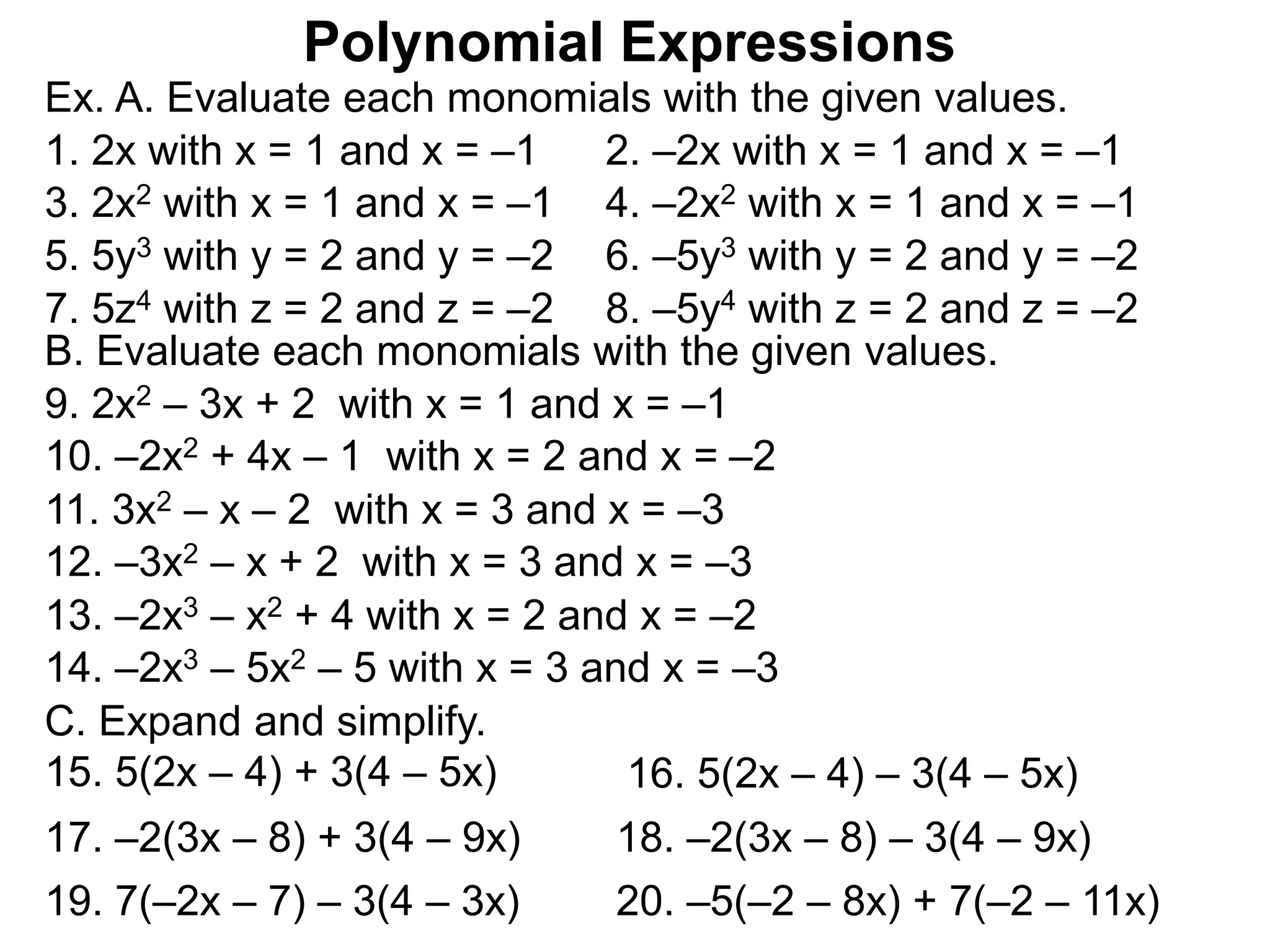
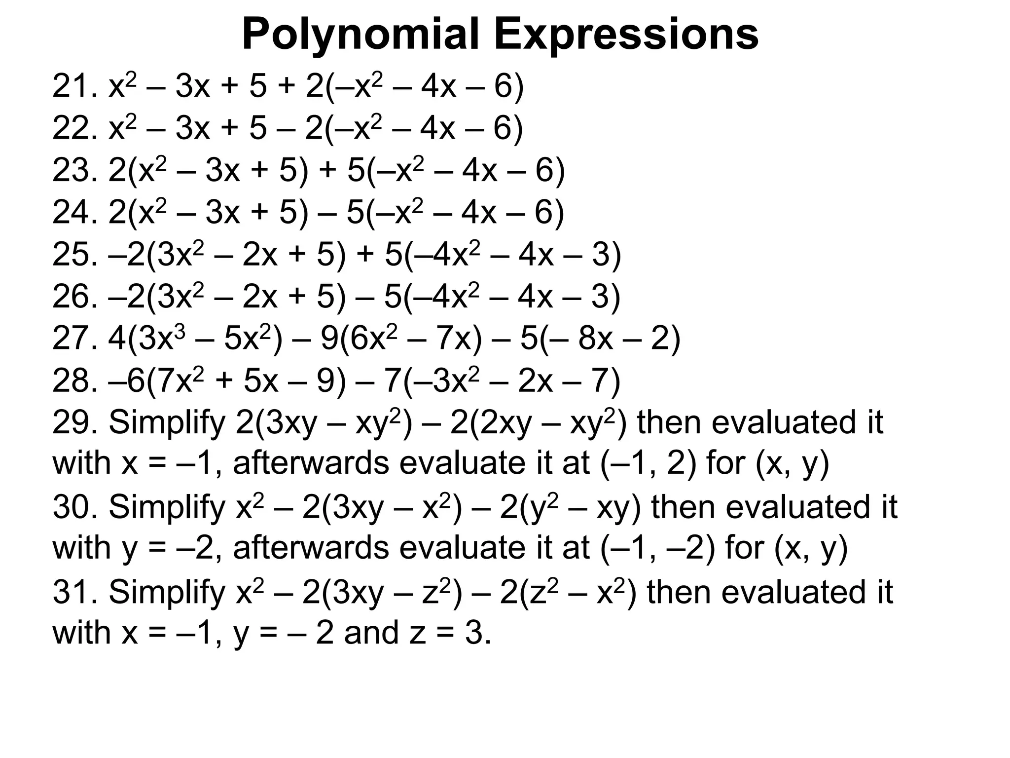
The document discusses polynomial expressions. A polynomial is the sum of monomial terms, where a monomial is a number multiplied by one or more variables raised to a non-negative integer power. Examples show evaluating polynomials by substituting values for variables and calculating each monomial term separately before combining them. A term refers to each monomial in a polynomial. Terms are identified by their variable part, such as the x2-term, x-term, or constant term.