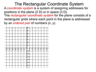
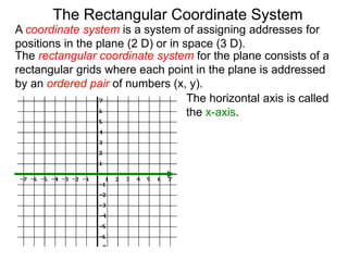
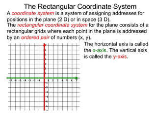
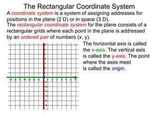
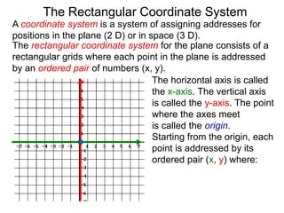
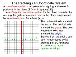
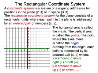
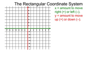
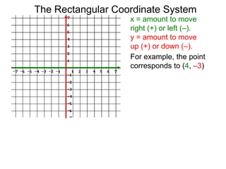
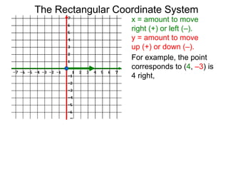
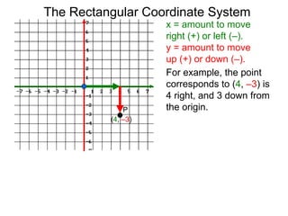
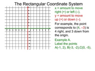
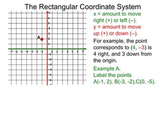
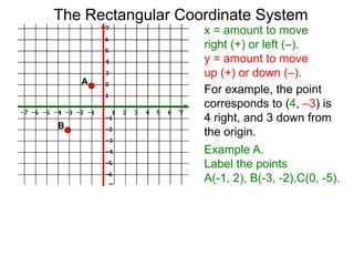
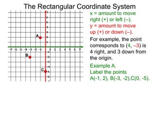
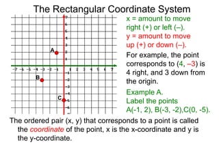
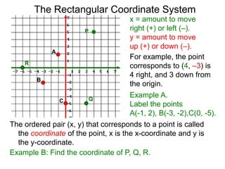
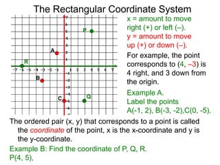
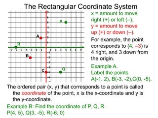
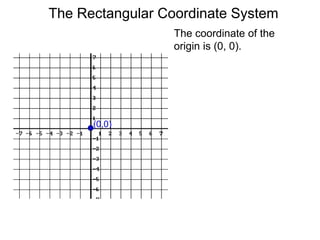
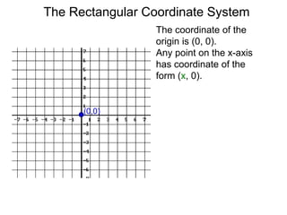
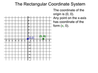
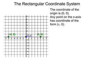
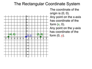
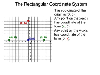
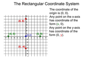
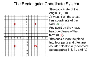
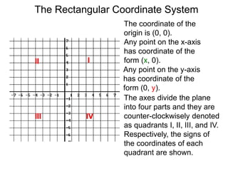
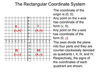
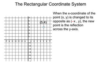
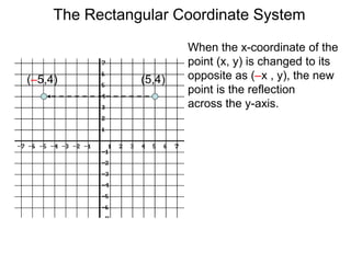
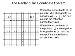
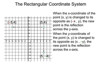
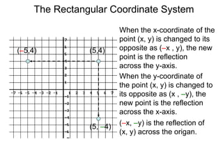
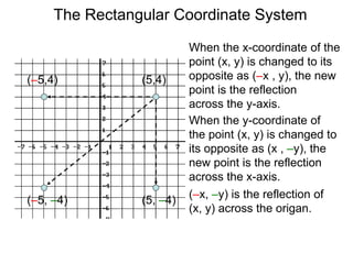
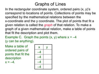
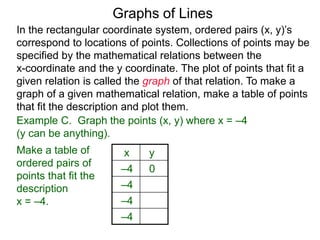
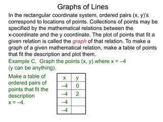
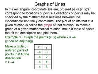
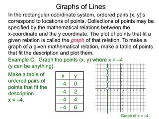
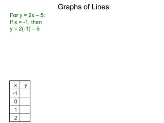
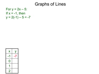
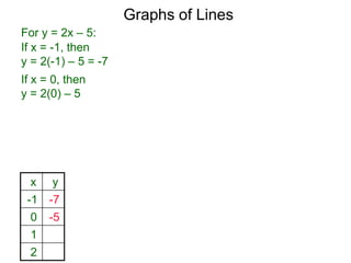
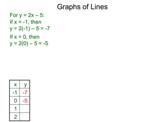
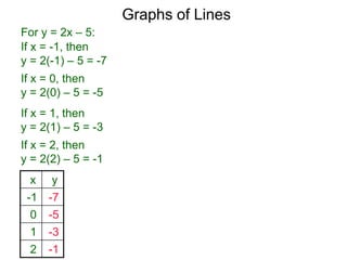
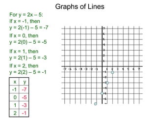
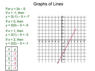
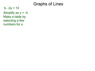
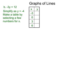
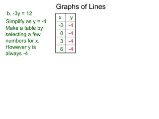
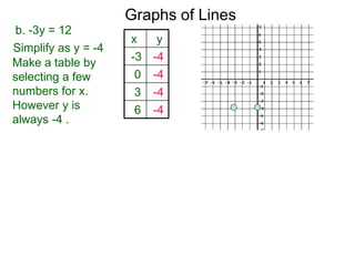
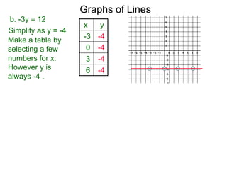
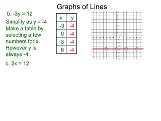
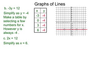
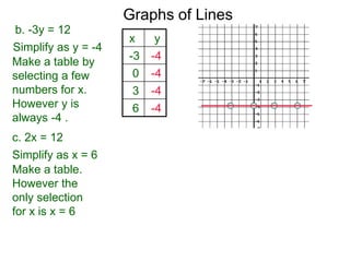
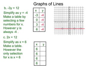
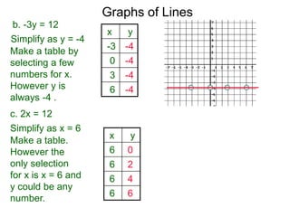
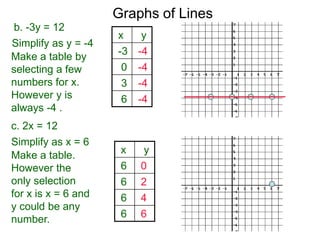
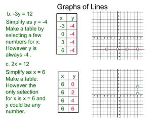
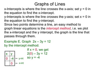
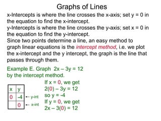
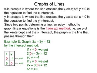
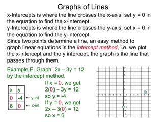
SlideShare a Scribd company logo
1 of 117
The Rectangular Coordinate System and Lines
Frank Ma Β© 2011
A coordinate system is a system of assigning addresses for
positions in the plane (2 D) or in space (3 D).
The Rectangular Coordinate System
A coordinate system is a system of assigning addresses for
positions in the plane (2 D) or in space (3 D).
The rectangular coordinate system for the plane consists of a
rectangular grids where each point in the plane is addressed
by an ordered pair of numbers (x, y).
The horizontal axis is called
the x-axis.
The Rectangular Coordinate System
A coordinate system is a system of assigning addresses for
positions in the plane (2 D) or in space (3 D).
The rectangular coordinate system for the plane consists of a
rectangular grids where each point in the plane is addressed
by an ordered pair of numbers (x, y).
The horizontal axis is called
the x-axis. The vertical axis
is called the y-axis.
The Rectangular Coordinate System
A coordinate system is a system of assigning addresses for
positions in the plane (2 D) or in space (3 D).
The rectangular coordinate system for the plane consists of a
rectangular grids where each point in the plane is addressed
by an ordered pair of numbers (x, y).
The horizontal axis is called
the x-axis. The vertical axis
is called the y-axis. The point
where the axes meet
is called the origin.
Starting from the origin, each
point is addressed by its
ordered pair (x, y) where:
x = amount to move
right (+) or left (–).
y = amount to move
up (+) or down (–).
The Rectangular Coordinate System
x = amount to move
right (+) or left (–).
y = amount to move
up (+) or down (–).
The Rectangular Coordinate System
x = amount to move
right (+) or left (–).
y = amount to move
up (+) or down (–).
For example, the point
corresponds to (4, –3)
The Rectangular Coordinate System
x = amount to move
right (+) or left (–).
y = amount to move
up (+) or down (–).
For example, the point
corresponds to (4, –3) is
4 right,
The Rectangular Coordinate System
x = amount to move
right (+) or left (–).
y = amount to move
up (+) or down (–).
For example, the point
corresponds to (4, –3) is
4 right, and 3 down from
the origin.
(4, –3)
P
The Rectangular Coordinate System
x = amount to move
right (+) or left (–).
y = amount to move
up (+) or down (–).
For example, the point
corresponds to (4, –3) is
4 right, and 3 down from
the origin.
Example A.
Label the points
A(-1, 2), B(-3, -2),C(0, -5).
The Rectangular Coordinate System
x = amount to move
right (+) or left (–).
y = amount to move
up (+) or down (–).
For example, the point
corresponds to (4, –3) is
4 right, and 3 down from
the origin.
Example A.
Label the points
A(-1, 2), B(-3, -2),C(0, -5).
A
The Rectangular Coordinate System
x = amount to move
right (+) or left (–).
y = amount to move
up (+) or down (–).
For example, the point
corresponds to (4, –3) is
4 right, and 3 down from
the origin.
Example A.
Label the points
A(-1, 2), B(-3, -2),C(0, -5).
A
B
The Rectangular Coordinate System
x = amount to move
right (+) or left (–).
y = amount to move
up (+) or down (–).
For example, the point
corresponds to (4, –3) is
4 right, and 3 down from
the origin.
Example A.
Label the points
A(-1, 2), B(-3, -2),C(0, -5).
A
B
C
The Rectangular Coordinate System
x = amount to move
right (+) or left (–).
y = amount to move
up (+) or down (–).
For example, the point
corresponds to (4, –3) is
4 right, and 3 down from
the origin.
Example A.
Label the points
A(-1, 2), B(-3, -2),C(0, -5).
The ordered pair (x, y) that corresponds to a point is called
the coordinate of the point, x is the x-coordinate and y is
the y-coordinate.
A
B
C
Example B: Find the coordinate of P, Q, R.
P
Q
R
The Rectangular Coordinate System
x = amount to move
right (+) or left (–).
y = amount to move
up (+) or down (–).
For example, the point
corresponds to (4, –3) is
4 right, and 3 down from
the origin.
Example A.
Label the points
A(-1, 2), B(-3, -2),C(0, -5).
The ordered pair (x, y) that corresponds to a point is called
the coordinate of the point, x is the x-coordinate and y is
the y-coordinate.
A
B
C
Example B: Find the coordinate of P, Q, R.
P(4, 5),
P
Q
R
The Rectangular Coordinate System
x = amount to move
right (+) or left (–).
y = amount to move
up (+) or down (–).
For example, the point
corresponds to (4, –3) is
4 right, and 3 down from
the origin.
Example A.
Label the points
A(-1, 2), B(-3, -2),C(0, -5).
The ordered pair (x, y) that corresponds to a point is called
the coordinate of the point, x is the x-coordinate and y is
the y-coordinate.
A
B
C
Example B: Find the coordinate of P, Q, R.
P(4, 5), Q(3, -5),
P
Q
R
The Rectangular Coordinate System
x = amount to move
right (+) or left (–).
y = amount to move
up (+) or down (–).
For example, the point
corresponds to (4, –3) is
4 right, and 3 down from
the origin.
Example A.
Label the points
A(-1, 2), B(-3, -2),C(0, -5).
The ordered pair (x, y) that corresponds to a point is called
the coordinate of the point, x is the x-coordinate and y is
the y-coordinate.
A
B
C
Example B: Find the coordinate of P, Q, R.
P(4, 5), Q(3, -5), R(-6, 0)
P
Q
R
The Rectangular Coordinate System
The coordinate of the
origin is (0, 0).
(0,0)
The Rectangular Coordinate System
The coordinate of the
origin is (0, 0).
Any point on the x-axis
has coordinate of the
form (x, 0).
(0,0)
The Rectangular Coordinate System
The coordinate of the
origin is (0, 0).
Any point on the x-axis
has coordinate of the
form (x, 0).
(5, 0)
(0,0)
The Rectangular Coordinate System
The coordinate of the
origin is (0, 0).
Any point on the x-axis
has coordinate of the
form (x, 0).
(5, 0)(-6, 0)
(0,0)
The Rectangular Coordinate System
The coordinate of the
origin is (0, 0).
Any point on the x-axis
has coordinate of the
form (x, 0).
(5, 0)(-6, 0)
Any point on the y-axis
has coordinate of the
form (0, y).(0,0)
The Rectangular Coordinate System
The coordinate of the
origin is (0, 0).
Any point on the x-axis
has coordinate of the
form (x, 0).
(5, 0)(-6, 0)
Any point on the y-axis
has coordinate of the
form (0, y).
(0, 6)
(0,0)
The Rectangular Coordinate System
The coordinate of the
origin is (0, 0).
Any point on the x-axis
has coordinate of the
form (x, 0).
(5, 0)(-6, 0)
Any point on the y-axis
has coordinate of the
form (0, y).
(0, -4)
(0, 6)
(0,0)
The Rectangular Coordinate System
The coordinate of the
origin is (0, 0).
Any point on the x-axis
has coordinate of the
form (x, 0).
Any point on the y-axis
has coordinate of the
form (0, y).
III
III IV
The axes divide the plane
into four parts and they are
counter-clockwisely denoted
as quadrants I, II, III, and IV.
The Rectangular Coordinate System
The coordinate of the
origin is (0, 0).
Any point on the x-axis
has coordinate of the
form (x, 0).
Any point on the y-axis
has coordinate of the
form (0, y).
The axes divide the plane
into four parts and they are
counter-clockwisely denoted
as quadrants I, II, III, and IV.
Respectively, the signs of
the coordinates of each
quadrant are shown.
III
III IV
(+,+)(–,+)
(–,–) (+,–)
The Rectangular Coordinate System
When the x-coordinate of the
point (x, y) is changed to its
opposite as (–x , y), the new
point is the reflection
across the y-axis.
(5,4)
The Rectangular Coordinate System
When the x-coordinate of the
point (x, y) is changed to its
opposite as (–x , y), the new
point is the reflection
across the y-axis.
(5,4)(–5,4)
The Rectangular Coordinate System
When the x-coordinate of the
point (x, y) is changed to its
opposite as (–x , y), the new
point is the reflection
across the y-axis.
When the y-coordinate of
the point (x, y) is changed to
its opposite as (x , –y), the
new point is the reflection
across the x-axis.
(5,4)(–5,4)
(5, –4)
(–x, –y) is the reflection of
(x, y) across the origan.
(–5, –4)
The Rectangular Coordinate System
Graphs of Lines
Graphs of Lines
In the rectangular coordinate system, ordered pairs (x, y)’s
correspond to locations of points.
Graphs of Lines
In the rectangular coordinate system, ordered pairs (x, y)’s
correspond to locations of points. Collections of points may be
specified by the mathematical relations between the
x-coordinate and the y coordinate.
Graphs of Lines
In the rectangular coordinate system, ordered pairs (x, y)’s
correspond to locations of points. Collections of points may be
specified by the mathematical relations between the
x-coordinate and the y coordinate. The plot of points that fit a
given relation is called the graph of that relation.
Graphs of Lines
In the rectangular coordinate system, ordered pairs (x, y)’s
correspond to locations of points. Collections of points may be
specified by the mathematical relations between the
x-coordinate and the y coordinate. The plot of points that fit a
given relation is called the graph of that relation. To make a
graph of a given mathematical relation, make a table of points
that fit the description and plot them.
Graphs of Lines
Example C. Graph the points (x, y) where x = –4
(y can be anything).
Make a table of
ordered pairs of
points that fit the
description
x = –4.
In the rectangular coordinate system, ordered pairs (x, y)’s
correspond to locations of points. Collections of points may be
specified by the mathematical relations between the
x-coordinate and the y coordinate. The plot of points that fit a
given relation is called the graph of that relation. To make a
graph of a given mathematical relation, make a table of points
that fit the description and plot them.
Graphs of Lines
Example C. Graph the points (x, y) where x = –4
(y can be anything).
x y
–4
–4
–4
–4
Make a table of
ordered pairs of
points that fit the
description
x = –4.
In the rectangular coordinate system, ordered pairs (x, y)’s
correspond to locations of points. Collections of points may be
specified by the mathematical relations between the
x-coordinate and the y coordinate. The plot of points that fit a
given relation is called the graph of that relation. To make a
graph of a given mathematical relation, make a table of points
that fit the description and plot them.
Graphs of Lines
Example C. Graph the points (x, y) where x = –4
(y can be anything).
x y
–4 0
–4
–4
–4
Make a table of
ordered pairs of
points that fit the
description
x = –4.
In the rectangular coordinate system, ordered pairs (x, y)’s
correspond to locations of points. Collections of points may be
specified by the mathematical relations between the
x-coordinate and the y coordinate. The plot of points that fit a
given relation is called the graph of that relation. To make a
graph of a given mathematical relation, make a table of points
that fit the description and plot them.
Graphs of Lines
Example C. Graph the points (x, y) where x = –4
(y can be anything).
x y
–4 0
–4 2
–4
–4
Make a table of
ordered pairs of
points that fit the
description
x = –4.
In the rectangular coordinate system, ordered pairs (x, y)’s
correspond to locations of points. Collections of points may be
specified by the mathematical relations between the
x-coordinate and the y coordinate. The plot of points that fit a
given relation is called the graph of that relation. To make a
graph of a given mathematical relation, make a table of points
that fit the description and plot them.
Graphs of Lines
Example C. Graph the points (x, y) where x = –4
(y can be anything).
x y
–4 0
–4 2
–4 4
–4 6
Graph of x = –4
Make a table of
ordered pairs of
points that fit the
description
x = –4.
In the rectangular coordinate system, ordered pairs (x, y)’s
correspond to locations of points. Collections of points may be
specified by the mathematical relations between the
x-coordinate and the y coordinate. The plot of points that fit a
given relation is called the graph of that relation. To make a
graph of a given mathematical relation, make a table of points
that fit the description and plot them.
Graphs of Lines
First degree equation in the variables x and y are equations
that may be put into the form Ax + By = C where A, B, C are
numbers.
Graphs of Lines
First degree equation in the variables x and y are equations
that may be put into the form Ax + By = C where A, B, C are
numbers. First degree equations are the same as linear
equations.
Graphs of Lines
First degree equation in the variables x and y are equations
that may be put into the form Ax + By = C where A, B, C are
numbers. First degree equations are the same as linear
equations. They are called linear because their graphs are
straight lines.
Graphs of Lines
First degree equation in the variables x and y are equations
that may be put into the form Ax + By = C where A, B, C are
numbers. First degree equations are the same as linear
equations. They are called linear because their graphs are
straight lines. To graph a linear equation, find a few ordered
pairs that fit the equation.
Graphs of Lines
First degree equation in the variables x and y are equations
that may be put into the form Ax + By = C where A, B, C are
numbers. First degree equations are the same as linear
equations. They are called linear because their graphs are
straight lines. To graph a linear equation, find a few ordered
pairs that fit the equation. To find one such ordered pair, assign
a value to x,
Graphs of Lines
First degree equation in the variables x and y are equations
that may be put into the form Ax + By = C where A, B, C are
numbers. First degree equations are the same as linear
equations. They are called linear because their graphs are
straight lines. To graph a linear equation, find a few ordered
pairs that fit the equation. To find one such ordered pair, assign
a value to x, plug it into the equation and solve for the y
(or assign a value to y and solve for the x).
Graphs of Lines
First degree equation in the variables x and y are equations
that may be put into the form Ax + By = C where A, B, C are
numbers. First degree equations are the same as linear
equations. They are called linear because their graphs are
straight lines. To graph a linear equation, find a few ordered
pairs that fit the equation. To find one such ordered pair, assign
a value to x, plug it into the equation and solve for the y
(or assign a value to y and solve for the x). For graphing lines,
find at least two ordered pairs.
Example D.
Graph the following linear equations.
a. y = 2x – 5
Make a table by selecting a few numbers for x.
Graphs of Lines
First degree equation in the variables x and y are equations
that may be put into the form Ax + By = C where A, B, C are
numbers. First degree equations are the same as linear
equations. They are called linear because their graphs are
straight lines. To graph a linear equation, find a few ordered
pairs that fit the equation. To find one such ordered pair, assign
a value to x, plug it into the equation and solve for the y
(or assign a value to y and solve for the x). For graphing lines,
find at least two ordered pairs.
Example D.
Graph the following linear equations.
a. y = 2x – 5
Make a table by selecting a few numbers for x. For easy
calculations we set x = -1, 0, 1, and 2.
Graphs of Lines
First degree equation in the variables x and y are equations
that may be put into the form Ax + By = C where A, B, C are
numbers. First degree equations are the same as linear
equations. They are called linear because their graphs are
straight lines. To graph a linear equation, find a few ordered
pairs that fit the equation. To find one such ordered pair, assign
a value to x, plug it into the equation and solve for the y
(or assign a value to y and solve for the x). For graphing lines,
find at least two ordered pairs.
Example D.
Graph the following linear equations.
a. y = 2x – 5
Make a table by selecting a few numbers for x. For easy
calculations we set x = -1, 0, 1, and 2. Plug each of these
values into x and find its corresponding y to form an ordered
pair.
Graphs of Lines
For y = 2x – 5:
x y
-1
0
1
2
Graphs of Lines
For y = 2x – 5:
x y
-1
0
1
2
If x = -1, then
y = 2(-1) – 5
Graphs of Lines
For y = 2x – 5:
x y
-1 -7
0
1
2
If x = -1, then
y = 2(-1) – 5 = -7
Graphs of Lines
For y = 2x – 5:
x y
-1 -7
0 -5
1
2
If x = -1, then
y = 2(-1) – 5 = -7
If x = 0, then
y = 2(0) – 5
Graphs of Lines
For y = 2x – 5:
x y
-1 -7
0 -5
1
2
If x = -1, then
y = 2(-1) – 5 = -7
If x = 0, then
y = 2(0) – 5 = -5
Graphs of Lines
For y = 2x – 5:
x y
-1 -7
0 -5
1 -3
2 -1
If x = -1, then
y = 2(-1) – 5 = -7
If x = 0, then
y = 2(0) – 5 = -5
If x = 1, then
y = 2(1) – 5 = -3
If x = 2, then
y = 2(2) – 5 = -1
Graphs of Lines
For y = 2x – 5:
x y
-1 -7
0 -5
1 -3
2 -1
If x = -1, then
y = 2(-1) – 5 = -7
If x = 0, then
y = 2(0) – 5 = -5
If x = 1, then
y = 2(1) – 5 = -3
If x = 2, then
y = 2(2) – 5 = -1
Graphs of Lines
For y = 2x – 5:
x y
-1 -7
0 -5
1 -3
2 -1
If x = -1, then
y = 2(-1) – 5 = -7
If x = 0, then
y = 2(0) – 5 = -5
If x = 1, then
y = 2(1) – 5 = -3
If x = 2, then
y = 2(2) – 5 = -1
Graphs of Lines
For y = 2x – 5:
x y
-1 -7
0 -5
1 -3
2 -1
If x = -1, then
y = 2(-1) – 5 = -7
If x = 0, then
y = 2(0) – 5 = -5
If x = 1, then
y = 2(1) – 5 = -3
If x = 2, then
y = 2(2) – 5 = -1
Graphs of Lines
For y = 2x – 5:
x y
-1 -7
0 -5
1 -3
2 -1
If x = -1, then
y = 2(-1) – 5 = -7
If x = 0, then
y = 2(0) – 5 = -5
If x = 1, then
y = 2(1) – 5 = -3
If x = 2, then
y = 2(2) – 5 = -1
Graphs of Lines
For y = 2x – 5:
x y
-1 -7
0 -5
1 -3
2 -1
If x = -1, then
y = 2(-1) – 5 = -7
If x = 0, then
y = 2(0) – 5 = -5
If x = 1, then
y = 2(1) – 5 = -3
If x = 2, then
y = 2(2) – 5 = -1
b. -3y = 12
Graphs of Lines
b. -3y = 12
Simplify as y = -4
Graphs of Lines
Make a table by
selecting a few
numbers for x.
b. -3y = 12
Simplify as y = -4
Graphs of Lines
Make a table by
selecting a few
numbers for x.
x y
-3
0
3
6
b. -3y = 12
Simplify as y = -4
Graphs of Lines
Make a table by
selecting a few
numbers for x.
However y is
always -4 .
x y
-3 -4
0 -4
3 -4
6 -4
b. -3y = 12
Simplify as y = -4
Graphs of Lines
Make a table by
selecting a few
numbers for x.
However y is
always -4 .
x y
-3 -4
0 -4
3 -4
6 -4
b. -3y = 12
Simplify as y = -4
Graphs of Lines
Make a table by
selecting a few
numbers for x.
However y is
always -4 .
x y
-3 -4
0 -4
3 -4
6 -4
b. -3y = 12
Simplify as y = -4
Graphs of Lines
Make a table by
selecting a few
numbers for x.
However y is
always -4 .
x y
-3 -4
0 -4
3 -4
6 -4
b. -3y = 12
Simplify as y = -4
Graphs of Lines
c. 2x = 12
Make a table by
selecting a few
numbers for x.
However y is
always -4 .
x y
-3 -4
0 -4
3 -4
6 -4
b. -3y = 12
Simplify as y = -4
Graphs of Lines
c. 2x = 12
Make a table by
selecting a few
numbers for x.
However y is
always -4 .
x y
-3 -4
0 -4
3 -4
6 -4
Simplify as x = 6.
b. -3y = 12
Simplify as y = -4
Graphs of Lines
c. 2x = 12
Make a table by
selecting a few
numbers for x.
However y is
always -4 .
x y
-3 -4
0 -4
3 -4
6 -4
Simplify as x = 6
Make a table.
However the
only selection
for x is x = 6
b. -3y = 12
Simplify as y = -4
Graphs of Lines
c. 2x = 12
Make a table by
selecting a few
numbers for x.
However y is
always -4 .
x y
-3 -4
0 -4
3 -4
6 -4
Simplify as x = 6
Make a table.
However the
only selection
for x is x = 6
x y
6
6
6
6
b. -3y = 12
Simplify as y = -4
Graphs of Lines
c. 2x = 12
Make a table by
selecting a few
numbers for x.
However y is
always -4 .
x y
-3 -4
0 -4
3 -4
6 -4
Simplify as x = 6
Make a table.
However the
only selection
for x is x = 6 and
y could be any
number.
x y
6 0
6 2
6 4
6 6
b. -3y = 12
Simplify as y = -4
Graphs of Lines
c. 2x = 12
Make a table by
selecting a few
numbers for x.
However y is
always -4 .
x y
-3 -4
0 -4
3 -4
6 -4
Simplify as x = 6
Make a table.
However the
only selection
for x is x = 6 and
y could be any
number.
x y
6 0
6 2
6 4
6 6
b. -3y = 12
Simplify as y = -4
Graphs of Lines
c. 2x = 12
Make a table by
selecting a few
numbers for x.
However y is
always -4 .
x y
-3 -4
0 -4
3 -4
6 -4
Simplify as x = 6
Make a table.
However the
only selection
for x is x = 6 and
y could be any
number.
x y
6 0
6 2
6 4
6 6
b. -3y = 12
Simplify as y = -4
Graphs of Lines
c. 2x = 12
Make a table by
selecting a few
numbers for x.
However y is
always -4 .
x y
-3 -4
0 -4
3 -4
6 -4
Simplify as x = 6
Make a table.
However the
only selection
for x is x = 6 and
y could be any
number.
x y
6 0
6 2
6 4
6 6
b. -3y = 12
Simplify as y = -4
Graphs of Lines
c. 2x = 12
Make a table by
selecting a few
numbers for x.
However y is
always -4 .
x y
-3 -4
0 -4
3 -4
6 -4
Simplify as x = 6
Make a table.
However the
only selection
for x is x = 6 and
y could be any
number.
x y
6 0
6 2
6 4
6 6
Summary of the graphs of linear equations:
Graphs of Lines
a. y = 2x – 5
Summary of the graphs of linear equations:
Graphs of Lines
a. y = 2x – 5
If both variables
x and y are
present in the
equation, the
graph is a
tilted line.
Summary of the graphs of linear equations:
Graphs of Lines
a. y = 2x – 5
If both variables
x and y are
present in the
equation, the
graph is a
tilted line.
Summary of the graphs of linear equations:
Graphs of Lines
a. y = 2x – 5 b. -3y = 12
If both variables
x and y are
present in the
equation, the
graph is a
tilted line.
Summary of the graphs of linear equations:
Graphs of Lines
a. y = 2x – 5 b. -3y = 12
If both variables
x and y are
present in the
equation, the
graph is a
tilted line.
If the equation has
only y (no x), the
graph is a
horizontal line.
Summary of the graphs of linear equations:
Graphs of Lines
a. y = 2x – 5 b. -3y = 12
If both variables
x and y are
present in the
equation, the
graph is a
tilted line.
If the equation has
only y (no x), the
graph is a
horizontal line.
Summary of the graphs of linear equations:
Graphs of Lines
a. y = 2x – 5 b. -3y = 12 c. 2x = 12
If both variables
x and y are
present in the
equation, the
graph is a
tilted line.
If the equation has
only y (no x), the
graph is a
horizontal line.
Summary of the graphs of linear equations:
Graphs of Lines
a. y = 2x – 5 b. -3y = 12 c. 2x = 12
If both variables
x and y are
present in the
equation, the
graph is a
tilted line.
If the equation has
only y (no x), the
graph is a
horizontal line.
Summary of the graphs of linear equations:
Graphs of Lines
If the equation has
only x (no y), the
graph is a
vertical line.
x-Intercepts is where the line crosses the x-axis;
Graphs of Lines
x-Intercepts is where the line crosses the x-axis; set y = 0 in
the equation to find the x-intercept.
Graphs of Lines
x-Intercepts is where the line crosses the x-axis; set y = 0 in
the equation to find the x-intercept.
y-Intercepts is where the line crosses the y-axis;
Graphs of Lines
x-Intercepts is where the line crosses the x-axis; set y = 0 in
the equation to find the x-intercept.
y-Intercepts is where the line crosses the y-axis; set x = 0 in
the equation to find the y-intercept.
Graphs of Lines
x-Intercepts is where the line crosses the x-axis; set y = 0 in
the equation to find the x-intercept.
y-Intercepts is where the line crosses the y-axis; set x = 0 in
the equation to find the y-intercept.
Graphs of Lines
Since two points determine a line, an easy method to
graph linear equations is the intercept method,
x-Intercepts is where the line crosses the x-axis; set y = 0 in
the equation to find the x-intercept.
y-Intercepts is where the line crosses the y-axis; set x = 0 in
the equation to find the y-intercept.
Graphs of Lines
Since two points determine a line, an easy method to
graph linear equations is the intercept method, i.e. we plot
the x-intercept and the y intercept, the graph is the line that
passes through them.
x-Intercepts is where the line crosses the x-axis; set y = 0 in
the equation to find the x-intercept.
y-Intercepts is where the line crosses the y-axis; set x = 0 in
the equation to find the y-intercept.
Graphs of Lines
Example E. Graph 2x – 3y = 12
by the intercept method.
Since two points determine a line, an easy method to
graph linear equations is the intercept method, i.e. we plot
the x-intercept and the y intercept, the graph is the line that
passes through them.
x y
0
0
x-Intercepts is where the line crosses the x-axis; set y = 0 in
the equation to find the x-intercept.
y-Intercepts is where the line crosses the y-axis; set x = 0 in
the equation to find the y-intercept.
y-int
x-int
Graphs of Lines
Example E. Graph 2x – 3y = 12
by the intercept method.
Since two points determine a line, an easy method to
graph linear equations is the intercept method, i.e. we plot
the x-intercept and the y intercept, the graph is the line that
passes through them.
If x = 0, we get
2(0) – 3y = 12
x y
0 -4
0
x-Intercepts is where the line crosses the x-axis; set y = 0 in
the equation to find the x-intercept.
y-Intercepts is where the line crosses the y-axis; set x = 0 in
the equation to find the y-intercept.
y-int
x-int
Graphs of Lines
Example E. Graph 2x – 3y = 12
by the intercept method.
Since two points determine a line, an easy method to
graph linear equations is the intercept method, i.e. we plot
the x-intercept and the y intercept, the graph is the line that
passes through them.
If x = 0, we get
2(0) – 3y = 12
so y = -4
If y = 0, we get
2x – 3(0) = 12
x y
0 -4
6 0
x-Intercepts is where the line crosses the x-axis; set y = 0 in
the equation to find the x-intercept.
y-Intercepts is where the line crosses the y-axis; set x = 0 in
the equation to find the y-intercept.
y-int
x-int
Graphs of Lines
Example E. Graph 2x – 3y = 12
by the intercept method.
Since two points determine a line, an easy method to
graph linear equations is the intercept method, i.e. we plot
the x-intercept and the y intercept, the graph is the line that
passes through them.
If x = 0, we get
2(0) – 3y = 12
so y = -4
If y = 0, we get
2x – 3(0) = 12
so x = 6
Exercise B. Graph the following equations. Identify the vertical
and the horizontal lines first. Then use the intercept method if
the method feasible.
9. x – y = 3 10. 2x = 6 11. –y – 7= 0
12. 0 = 8 – 2x 13. y = –x + 4 14. 2x – 3 = 6
15. 2x = 6 – 2y 16. 4y – 12 = 3x 17. –2x + 3y = 3
18. –6 = 3x – 2y 19. 3x + 2 = 4y + 3x 20. 5x + 2y = –10
The Rectangular Coordinate System and Lines
Exercise A. Starting at (3, 4), find the coordinate of the point if
we move. Draw the points.
1. 2 units up, 2 units right. 2. 2 units up, 2 units left.
3. 2 units down, 2 units right. 4. 2 units down, 2 units left.
Starting at (–3, 4), find the coordinate of the point if we move.
Draw the points.
6. 7 units up, 9 units right.5. 12 units up, 4 units left.
7. 7 units down, 6 units right. 8. 11 units down, 7 units left.

More Related Content

What's hot

59 constructing linea equations of lines
59 constructing linea equations of lines59 constructing linea equations of lines
59 constructing linea equations of linesalg1testreview
Β 
10 rectangular coordinate system x
10 rectangular coordinate system x10 rectangular coordinate system x
10 rectangular coordinate system xmath260
Β 
8 sign charts of factorable formulas y
8 sign charts of factorable formulas y8 sign charts of factorable formulas y
8 sign charts of factorable formulas ymath260
Β 
Graphing parabola presentation
Graphing parabola presentationGraphing parabola presentation
Graphing parabola presentationVirgilio Paragele
Β 
Notes parabolas
Notes   parabolasNotes   parabolas
Notes parabolasLori Rapp
Β 
2.0 rectangular coordinate system t
2.0 rectangular coordinate system t2.0 rectangular coordinate system t
2.0 rectangular coordinate system tmath260
Β 
57 graphing lines from linear equations
57 graphing lines from linear equations57 graphing lines from linear equations
57 graphing lines from linear equationsalg1testreview
Β 
13 graphs of factorable polynomials x
13 graphs of factorable polynomials x13 graphs of factorable polynomials x
13 graphs of factorable polynomials xmath260
Β 
Parabola complete
Parabola completeParabola complete
Parabola completeMATOME PETER
Β 
1.2 the graphs of quadratic equations
1.2 the graphs of quadratic equations1.2 the graphs of quadratic equations
1.2 the graphs of quadratic equationsmath123c
Β 
11 graphs of first degree functions x
11 graphs of first degree functions x11 graphs of first degree functions x
11 graphs of first degree functions xmath260
Β 
Parabola 091102134314-phpapp01
Parabola 091102134314-phpapp01Parabola 091102134314-phpapp01
Parabola 091102134314-phpapp01A.
Β 
7 sign charts and inequalities i x
7 sign charts and inequalities i x7 sign charts and inequalities i x
7 sign charts and inequalities i xmath260
Β 
Properties of Parabola
Properties of ParabolaProperties of Parabola
Properties of Parabolarey castro
Β 
1 polar coordinates
1 polar coordinates1 polar coordinates
1 polar coordinatesmath267
Β 
Conic sections
Conic sectionsConic sections
Conic sectionsfaizy8622
Β 
12 graphs of second degree functions x
12 graphs of second degree functions x12 graphs of second degree functions x
12 graphs of second degree functions xmath260
Β 

What's hot (20)

59 constructing linea equations of lines
59 constructing linea equations of lines59 constructing linea equations of lines
59 constructing linea equations of lines
Β 
10 rectangular coordinate system x
10 rectangular coordinate system x10 rectangular coordinate system x
10 rectangular coordinate system x
Β 
1576 parabola
1576 parabola1576 parabola
1576 parabola
Β 
8 sign charts of factorable formulas y
8 sign charts of factorable formulas y8 sign charts of factorable formulas y
8 sign charts of factorable formulas y
Β 
Parabola
ParabolaParabola
Parabola
Β 
Graphing parabola presentation
Graphing parabola presentationGraphing parabola presentation
Graphing parabola presentation
Β 
Notes parabolas
Notes   parabolasNotes   parabolas
Notes parabolas
Β 
2.0 rectangular coordinate system t
2.0 rectangular coordinate system t2.0 rectangular coordinate system t
2.0 rectangular coordinate system t
Β 
57 graphing lines from linear equations
57 graphing lines from linear equations57 graphing lines from linear equations
57 graphing lines from linear equations
Β 
13 graphs of factorable polynomials x
13 graphs of factorable polynomials x13 graphs of factorable polynomials x
13 graphs of factorable polynomials x
Β 
Parabola complete
Parabola completeParabola complete
Parabola complete
Β 
1.2 the graphs of quadratic equations
1.2 the graphs of quadratic equations1.2 the graphs of quadratic equations
1.2 the graphs of quadratic equations
Β 
11 graphs of first degree functions x
11 graphs of first degree functions x11 graphs of first degree functions x
11 graphs of first degree functions x
Β 
Parabola 091102134314-phpapp01
Parabola 091102134314-phpapp01Parabola 091102134314-phpapp01
Parabola 091102134314-phpapp01
Β 
7 sign charts and inequalities i x
7 sign charts and inequalities i x7 sign charts and inequalities i x
7 sign charts and inequalities i x
Β 
Properties of Parabola
Properties of ParabolaProperties of Parabola
Properties of Parabola
Β 
Parabola
ParabolaParabola
Parabola
Β 
1 polar coordinates
1 polar coordinates1 polar coordinates
1 polar coordinates
Β 
Conic sections
Conic sectionsConic sections
Conic sections
Β 
12 graphs of second degree functions x
12 graphs of second degree functions x12 graphs of second degree functions x
12 graphs of second degree functions x
Β 

Similar to 4 linear equations and graphs of lines

1 rectangular coordinate system x
1 rectangular coordinate system x1 rectangular coordinate system x
1 rectangular coordinate system xTzenma
Β 
Coordinate System.pptx
Coordinate System.pptxCoordinate System.pptx
Coordinate System.pptxKeizylleCajeme
Β 
Coordinate System.pptx
Coordinate System.pptxCoordinate System.pptx
Coordinate System.pptxKeizylleCajeme
Β 
267 1 3 d coordinate system-n
267 1 3 d coordinate system-n267 1 3 d coordinate system-n
267 1 3 d coordinate system-nmath266
Β 
267 1 3 d coordinate system-n
267 1 3 d coordinate system-n267 1 3 d coordinate system-n
267 1 3 d coordinate system-nmath260
Β 
Coordinate geometry 9 grade
Coordinate geometry 9 gradeCoordinate geometry 9 grade
Coordinate geometry 9 gradeSiddu Lingesh
Β 
linear equations in two variables
linear equations in two variableslinear equations in two variables
linear equations in two variablesMpumi Mokoena
Β 
linear equation in 2 variables
linear equation in 2 variableslinear equation in 2 variables
linear equation in 2 variablesmukundapriya
Β 
1 3 d coordinate system
1 3 d coordinate system1 3 d coordinate system
1 3 d coordinate systemmath267
Β 
27 triple integrals in spherical and cylindrical coordinates
27 triple integrals in spherical and cylindrical coordinates27 triple integrals in spherical and cylindrical coordinates
27 triple integrals in spherical and cylindrical coordinatesmath267
Β 
Geometry (Grid & section formula)
Geometry (Grid & section formula)Geometry (Grid & section formula)
Geometry (Grid & section formula)itutor
Β 
Cordinate geometry for class VIII and IX
Cordinate  geometry for class VIII and IXCordinate  geometry for class VIII and IX
Cordinate geometry for class VIII and IXMD. G R Ahmed
Β 
The rectangular coordinate plane
The rectangular coordinate planeThe rectangular coordinate plane
The rectangular coordinate planeMartinGeraldine
Β 
Linear equation in 2 variables
Linear equation in 2 variablesLinear equation in 2 variables
Linear equation in 2 variablesavb public school
Β 
EMT_2A_cylindrical coordinates.pptx
EMT_2A_cylindrical coordinates.pptxEMT_2A_cylindrical coordinates.pptx
EMT_2A_cylindrical coordinates.pptx5610UmarIqbal
Β 
Analytic geometry basic concepts
Analytic geometry basic conceptsAnalytic geometry basic concepts
Analytic geometry basic conceptsNancy Morales Felipe
Β 

Similar to 4 linear equations and graphs of lines (20)

1 rectangular coordinate system x
1 rectangular coordinate system x1 rectangular coordinate system x
1 rectangular coordinate system x
Β 
Coordinate System.pptx
Coordinate System.pptxCoordinate System.pptx
Coordinate System.pptx
Β 
Coordinate System.pptx
Coordinate System.pptxCoordinate System.pptx
Coordinate System.pptx
Β 
267 1 3 d coordinate system-n
267 1 3 d coordinate system-n267 1 3 d coordinate system-n
267 1 3 d coordinate system-n
Β 
267 1 3 d coordinate system-n
267 1 3 d coordinate system-n267 1 3 d coordinate system-n
267 1 3 d coordinate system-n
Β 
Coordinate geometry 9 grade
Coordinate geometry 9 gradeCoordinate geometry 9 grade
Coordinate geometry 9 grade
Β 
linear equations in two variables
linear equations in two variableslinear equations in two variables
linear equations in two variables
Β 
linear equation in 2 variables
linear equation in 2 variableslinear equation in 2 variables
linear equation in 2 variables
Β 
1 3 d coordinate system
1 3 d coordinate system1 3 d coordinate system
1 3 d coordinate system
Β 
27 triple integrals in spherical and cylindrical coordinates
27 triple integrals in spherical and cylindrical coordinates27 triple integrals in spherical and cylindrical coordinates
27 triple integrals in spherical and cylindrical coordinates
Β 
Geometry (Grid & section formula)
Geometry (Grid & section formula)Geometry (Grid & section formula)
Geometry (Grid & section formula)
Β 
Cordinate geometry for class VIII and IX
Cordinate  geometry for class VIII and IXCordinate  geometry for class VIII and IX
Cordinate geometry for class VIII and IX
Β 
Msm1 fl ch11_03
Msm1 fl ch11_03Msm1 fl ch11_03
Msm1 fl ch11_03
Β 
Msm1 fl ch11_03
Msm1 fl ch11_03Msm1 fl ch11_03
Msm1 fl ch11_03
Β 
1 6 Notes
1 6 Notes1 6 Notes
1 6 Notes
Β 
The rectangular coordinate plane
The rectangular coordinate planeThe rectangular coordinate plane
The rectangular coordinate plane
Β 
Linear equation in 2 variables
Linear equation in 2 variablesLinear equation in 2 variables
Linear equation in 2 variables
Β 
EMT_2A_cylindrical coordinates.pptx
EMT_2A_cylindrical coordinates.pptxEMT_2A_cylindrical coordinates.pptx
EMT_2A_cylindrical coordinates.pptx
Β 
Coordinate geometry
Coordinate geometryCoordinate geometry
Coordinate geometry
Β 
Analytic geometry basic concepts
Analytic geometry basic conceptsAnalytic geometry basic concepts
Analytic geometry basic concepts
Β 

More from elem-alg-sample

6 equations and applications of lines
6 equations and applications of lines6 equations and applications of lines
6 equations and applications of lineselem-alg-sample
Β 
2 the real line, inequalities and comparative phrases
2 the real line, inequalities and comparative phrases2 the real line, inequalities and comparative phrases
2 the real line, inequalities and comparative phraseselem-alg-sample
Β 
1 basic geometry and formulas
1 basic geometry and formulas1 basic geometry and formulas
1 basic geometry and formulaselem-alg-sample
Β 
17 applications of proportions and the rational equations
17 applications of proportions and the rational equations17 applications of proportions and the rational equations
17 applications of proportions and the rational equationselem-alg-sample
Β 
16 the multiplier method for simplifying complex fractions
16 the multiplier method for simplifying complex fractions16 the multiplier method for simplifying complex fractions
16 the multiplier method for simplifying complex fractionselem-alg-sample
Β 
15 proportions and the multiplier method for solving rational equations
15 proportions and the multiplier method for solving rational equations15 proportions and the multiplier method for solving rational equations
15 proportions and the multiplier method for solving rational equationselem-alg-sample
Β 
14 the lcm and the multiplier method for addition and subtraction of rational...
14 the lcm and the multiplier method for addition and subtraction of rational...14 the lcm and the multiplier method for addition and subtraction of rational...
14 the lcm and the multiplier method for addition and subtraction of rational...elem-alg-sample
Β 
13 multiplication and division of rational expressions
13 multiplication and division of rational expressions13 multiplication and division of rational expressions
13 multiplication and division of rational expressionselem-alg-sample
Β 
12 rational expressions
12 rational expressions12 rational expressions
12 rational expressionselem-alg-sample
Β 
11 applications of factoring
11 applications of factoring11 applications of factoring
11 applications of factoringelem-alg-sample
Β 
10 more on factoring trinomials and factoring by formulas
10 more on factoring trinomials and factoring by formulas10 more on factoring trinomials and factoring by formulas
10 more on factoring trinomials and factoring by formulaselem-alg-sample
Β 
9 factoring trinomials
9 factoring trinomials9 factoring trinomials
9 factoring trinomialselem-alg-sample
Β 
8 factoring out gcf
8 factoring out gcf8 factoring out gcf
8 factoring out gcfelem-alg-sample
Β 
7 special binomial operations and formulas
7 special binomial operations and formulas7 special binomial operations and formulas
7 special binomial operations and formulaselem-alg-sample
Β 
6 polynomial expressions and operations
6 polynomial expressions and operations6 polynomial expressions and operations
6 polynomial expressions and operationselem-alg-sample
Β 
5 exponents and scientific notation
5 exponents and scientific notation5 exponents and scientific notation
5 exponents and scientific notationelem-alg-sample
Β 
4 literal equations
4 literal equations4 literal equations
4 literal equationselem-alg-sample
Β 
3 linear equations
3 linear equations3 linear equations
3 linear equationselem-alg-sample
Β 

More from elem-alg-sample (20)

6 equations and applications of lines
6 equations and applications of lines6 equations and applications of lines
6 equations and applications of lines
Β 
5 slopes of lines
5 slopes of lines5 slopes of lines
5 slopes of lines
Β 
2 the real line, inequalities and comparative phrases
2 the real line, inequalities and comparative phrases2 the real line, inequalities and comparative phrases
2 the real line, inequalities and comparative phrases
Β 
1 basic geometry and formulas
1 basic geometry and formulas1 basic geometry and formulas
1 basic geometry and formulas
Β 
18 variations
18 variations18 variations
18 variations
Β 
17 applications of proportions and the rational equations
17 applications of proportions and the rational equations17 applications of proportions and the rational equations
17 applications of proportions and the rational equations
Β 
16 the multiplier method for simplifying complex fractions
16 the multiplier method for simplifying complex fractions16 the multiplier method for simplifying complex fractions
16 the multiplier method for simplifying complex fractions
Β 
15 proportions and the multiplier method for solving rational equations
15 proportions and the multiplier method for solving rational equations15 proportions and the multiplier method for solving rational equations
15 proportions and the multiplier method for solving rational equations
Β 
14 the lcm and the multiplier method for addition and subtraction of rational...
14 the lcm and the multiplier method for addition and subtraction of rational...14 the lcm and the multiplier method for addition and subtraction of rational...
14 the lcm and the multiplier method for addition and subtraction of rational...
Β 
13 multiplication and division of rational expressions
13 multiplication and division of rational expressions13 multiplication and division of rational expressions
13 multiplication and division of rational expressions
Β 
12 rational expressions
12 rational expressions12 rational expressions
12 rational expressions
Β 
11 applications of factoring
11 applications of factoring11 applications of factoring
11 applications of factoring
Β 
10 more on factoring trinomials and factoring by formulas
10 more on factoring trinomials and factoring by formulas10 more on factoring trinomials and factoring by formulas
10 more on factoring trinomials and factoring by formulas
Β 
9 factoring trinomials
9 factoring trinomials9 factoring trinomials
9 factoring trinomials
Β 
8 factoring out gcf
8 factoring out gcf8 factoring out gcf
8 factoring out gcf
Β 
7 special binomial operations and formulas
7 special binomial operations and formulas7 special binomial operations and formulas
7 special binomial operations and formulas
Β 
6 polynomial expressions and operations
6 polynomial expressions and operations6 polynomial expressions and operations
6 polynomial expressions and operations
Β 
5 exponents and scientific notation
5 exponents and scientific notation5 exponents and scientific notation
5 exponents and scientific notation
Β 
4 literal equations
4 literal equations4 literal equations
4 literal equations
Β 
3 linear equations
3 linear equations3 linear equations
3 linear equations
Β 

Recently uploaded

Interactive Powerpoint_How to Master effective communication
Interactive Powerpoint_How to Master effective communicationInteractive Powerpoint_How to Master effective communication
Interactive Powerpoint_How to Master effective communicationnomboosow
Β 
MENTAL STATUS EXAMINATION format.docx
MENTAL     STATUS EXAMINATION format.docxMENTAL     STATUS EXAMINATION format.docx
MENTAL STATUS EXAMINATION format.docxPoojaSen20
Β 
Solving Puzzles Benefits Everyone (English).pptx
Solving Puzzles Benefits Everyone (English).pptxSolving Puzzles Benefits Everyone (English).pptx
Solving Puzzles Benefits Everyone (English).pptxOH TEIK BIN
Β 
Software Engineering Methodologies (overview)
Software Engineering Methodologies (overview)Software Engineering Methodologies (overview)
Software Engineering Methodologies (overview)eniolaolutunde
Β 
Enzyme, Pharmaceutical Aids, Miscellaneous Last Part of Chapter no 5th.pdf
Enzyme, Pharmaceutical Aids, Miscellaneous Last Part of Chapter no 5th.pdfEnzyme, Pharmaceutical Aids, Miscellaneous Last Part of Chapter no 5th.pdf
Enzyme, Pharmaceutical Aids, Miscellaneous Last Part of Chapter no 5th.pdfSumit Tiwari
Β 
_Math 4-Q4 Week 5.pptx Steps in Collecting Data
_Math 4-Q4 Week 5.pptx Steps in Collecting Data_Math 4-Q4 Week 5.pptx Steps in Collecting Data
_Math 4-Q4 Week 5.pptx Steps in Collecting DataJhengPantaleon
Β 
β€œOh GOSH! Reflecting on Hackteria's Collaborative Practices in a Global Do-It...
β€œOh GOSH! Reflecting on Hackteria's Collaborative Practices in a Global Do-It...β€œOh GOSH! Reflecting on Hackteria's Collaborative Practices in a Global Do-It...
β€œOh GOSH! Reflecting on Hackteria's Collaborative Practices in a Global Do-It...Marc Dusseiller Dusjagr
Β 
How to Configure Email Server in Odoo 17
How to Configure Email Server in Odoo 17How to Configure Email Server in Odoo 17
How to Configure Email Server in Odoo 17Celine George
Β 
BASLIQ CURRENT LOOKBOOK LOOKBOOK(1) (1).pdf
BASLIQ CURRENT LOOKBOOK  LOOKBOOK(1) (1).pdfBASLIQ CURRENT LOOKBOOK  LOOKBOOK(1) (1).pdf
BASLIQ CURRENT LOOKBOOK LOOKBOOK(1) (1).pdfSoniaTolstoy
Β 
Contemporary philippine arts from the regions_PPT_Module_12 [Autosaved] (1).pptx
Contemporary philippine arts from the regions_PPT_Module_12 [Autosaved] (1).pptxContemporary philippine arts from the regions_PPT_Module_12 [Autosaved] (1).pptx
Contemporary philippine arts from the regions_PPT_Module_12 [Autosaved] (1).pptxRoyAbrique
Β 
Incoming and Outgoing Shipments in 1 STEP Using Odoo 17
Incoming and Outgoing Shipments in 1 STEP Using Odoo 17Incoming and Outgoing Shipments in 1 STEP Using Odoo 17
Incoming and Outgoing Shipments in 1 STEP Using Odoo 17Celine George
Β 
KSHARA STURA .pptx---KSHARA KARMA THERAPY (CAUSTIC THERAPY)β€”β€”β€”β€”IMP.OF KSHARA ...
KSHARA STURA .pptx---KSHARA KARMA THERAPY (CAUSTIC THERAPY)β€”β€”β€”β€”IMP.OF KSHARA ...KSHARA STURA .pptx---KSHARA KARMA THERAPY (CAUSTIC THERAPY)β€”β€”β€”β€”IMP.OF KSHARA ...
KSHARA STURA .pptx---KSHARA KARMA THERAPY (CAUSTIC THERAPY)β€”β€”β€”β€”IMP.OF KSHARA ...M56BOOKSTORE PRODUCT/SERVICE
Β 
Mastering the Unannounced Regulatory Inspection
Mastering the Unannounced Regulatory InspectionMastering the Unannounced Regulatory Inspection
Mastering the Unannounced Regulatory InspectionSafetyChain Software
Β 
Organic Name Reactions for the students and aspirants of Chemistry12th.pptx
Organic Name Reactions  for the students and aspirants of Chemistry12th.pptxOrganic Name Reactions  for the students and aspirants of Chemistry12th.pptx
Organic Name Reactions for the students and aspirants of Chemistry12th.pptxVS Mahajan Coaching Centre
Β 
Kisan Call Centre - To harness potential of ICT in Agriculture by answer farm...
Kisan Call Centre - To harness potential of ICT in Agriculture by answer farm...Kisan Call Centre - To harness potential of ICT in Agriculture by answer farm...
Kisan Call Centre - To harness potential of ICT in Agriculture by answer farm...Krashi Coaching
Β 
call girls in Kamla Market (DELHI) πŸ” >ΰΌ’9953330565πŸ” genuine Escort Service πŸ”βœ”οΈβœ”οΈ
call girls in Kamla Market (DELHI) πŸ” >ΰΌ’9953330565πŸ” genuine Escort Service πŸ”βœ”οΈβœ”οΈcall girls in Kamla Market (DELHI) πŸ” >ΰΌ’9953330565πŸ” genuine Escort Service πŸ”βœ”οΈβœ”οΈ
call girls in Kamla Market (DELHI) πŸ” >ΰΌ’9953330565πŸ” genuine Escort Service πŸ”βœ”οΈβœ”οΈ9953056974 Low Rate Call Girls In Saket, Delhi NCR
Β 
Introduction to AI in Higher Education_draft.pptx
Introduction to AI in Higher Education_draft.pptxIntroduction to AI in Higher Education_draft.pptx
Introduction to AI in Higher Education_draft.pptxpboyjonauth
Β 

Recently uploaded (20)

Model Call Girl in Bikash Puri Delhi reach out to us at πŸ”9953056974πŸ”
Model Call Girl in Bikash Puri  Delhi reach out to us at πŸ”9953056974πŸ”Model Call Girl in Bikash Puri  Delhi reach out to us at πŸ”9953056974πŸ”
Model Call Girl in Bikash Puri Delhi reach out to us at πŸ”9953056974πŸ”
Β 
Interactive Powerpoint_How to Master effective communication
Interactive Powerpoint_How to Master effective communicationInteractive Powerpoint_How to Master effective communication
Interactive Powerpoint_How to Master effective communication
Β 
MENTAL STATUS EXAMINATION format.docx
MENTAL     STATUS EXAMINATION format.docxMENTAL     STATUS EXAMINATION format.docx
MENTAL STATUS EXAMINATION format.docx
Β 
Solving Puzzles Benefits Everyone (English).pptx
Solving Puzzles Benefits Everyone (English).pptxSolving Puzzles Benefits Everyone (English).pptx
Solving Puzzles Benefits Everyone (English).pptx
Β 
Software Engineering Methodologies (overview)
Software Engineering Methodologies (overview)Software Engineering Methodologies (overview)
Software Engineering Methodologies (overview)
Β 
Model Call Girl in Tilak Nagar Delhi reach out to us at πŸ”9953056974πŸ”
Model Call Girl in Tilak Nagar Delhi reach out to us at πŸ”9953056974πŸ”Model Call Girl in Tilak Nagar Delhi reach out to us at πŸ”9953056974πŸ”
Model Call Girl in Tilak Nagar Delhi reach out to us at πŸ”9953056974πŸ”
Β 
Enzyme, Pharmaceutical Aids, Miscellaneous Last Part of Chapter no 5th.pdf
Enzyme, Pharmaceutical Aids, Miscellaneous Last Part of Chapter no 5th.pdfEnzyme, Pharmaceutical Aids, Miscellaneous Last Part of Chapter no 5th.pdf
Enzyme, Pharmaceutical Aids, Miscellaneous Last Part of Chapter no 5th.pdf
Β 
_Math 4-Q4 Week 5.pptx Steps in Collecting Data
_Math 4-Q4 Week 5.pptx Steps in Collecting Data_Math 4-Q4 Week 5.pptx Steps in Collecting Data
_Math 4-Q4 Week 5.pptx Steps in Collecting Data
Β 
β€œOh GOSH! Reflecting on Hackteria's Collaborative Practices in a Global Do-It...
β€œOh GOSH! Reflecting on Hackteria's Collaborative Practices in a Global Do-It...β€œOh GOSH! Reflecting on Hackteria's Collaborative Practices in a Global Do-It...
β€œOh GOSH! Reflecting on Hackteria's Collaborative Practices in a Global Do-It...
Β 
How to Configure Email Server in Odoo 17
How to Configure Email Server in Odoo 17How to Configure Email Server in Odoo 17
How to Configure Email Server in Odoo 17
Β 
BASLIQ CURRENT LOOKBOOK LOOKBOOK(1) (1).pdf
BASLIQ CURRENT LOOKBOOK  LOOKBOOK(1) (1).pdfBASLIQ CURRENT LOOKBOOK  LOOKBOOK(1) (1).pdf
BASLIQ CURRENT LOOKBOOK LOOKBOOK(1) (1).pdf
Β 
Contemporary philippine arts from the regions_PPT_Module_12 [Autosaved] (1).pptx
Contemporary philippine arts from the regions_PPT_Module_12 [Autosaved] (1).pptxContemporary philippine arts from the regions_PPT_Module_12 [Autosaved] (1).pptx
Contemporary philippine arts from the regions_PPT_Module_12 [Autosaved] (1).pptx
Β 
Incoming and Outgoing Shipments in 1 STEP Using Odoo 17
Incoming and Outgoing Shipments in 1 STEP Using Odoo 17Incoming and Outgoing Shipments in 1 STEP Using Odoo 17
Incoming and Outgoing Shipments in 1 STEP Using Odoo 17
Β 
KSHARA STURA .pptx---KSHARA KARMA THERAPY (CAUSTIC THERAPY)β€”β€”β€”β€”IMP.OF KSHARA ...
KSHARA STURA .pptx---KSHARA KARMA THERAPY (CAUSTIC THERAPY)β€”β€”β€”β€”IMP.OF KSHARA ...KSHARA STURA .pptx---KSHARA KARMA THERAPY (CAUSTIC THERAPY)β€”β€”β€”β€”IMP.OF KSHARA ...
KSHARA STURA .pptx---KSHARA KARMA THERAPY (CAUSTIC THERAPY)β€”β€”β€”β€”IMP.OF KSHARA ...
Β 
Mastering the Unannounced Regulatory Inspection
Mastering the Unannounced Regulatory InspectionMastering the Unannounced Regulatory Inspection
Mastering the Unannounced Regulatory Inspection
Β 
Organic Name Reactions for the students and aspirants of Chemistry12th.pptx
Organic Name Reactions  for the students and aspirants of Chemistry12th.pptxOrganic Name Reactions  for the students and aspirants of Chemistry12th.pptx
Organic Name Reactions for the students and aspirants of Chemistry12th.pptx
Β 
9953330565 Low Rate Call Girls In Rohini Delhi NCR
9953330565 Low Rate Call Girls In Rohini  Delhi NCR9953330565 Low Rate Call Girls In Rohini  Delhi NCR
9953330565 Low Rate Call Girls In Rohini Delhi NCR
Β 
Kisan Call Centre - To harness potential of ICT in Agriculture by answer farm...
Kisan Call Centre - To harness potential of ICT in Agriculture by answer farm...Kisan Call Centre - To harness potential of ICT in Agriculture by answer farm...
Kisan Call Centre - To harness potential of ICT in Agriculture by answer farm...
Β 
call girls in Kamla Market (DELHI) πŸ” >ΰΌ’9953330565πŸ” genuine Escort Service πŸ”βœ”οΈβœ”οΈ
call girls in Kamla Market (DELHI) πŸ” >ΰΌ’9953330565πŸ” genuine Escort Service πŸ”βœ”οΈβœ”οΈcall girls in Kamla Market (DELHI) πŸ” >ΰΌ’9953330565πŸ” genuine Escort Service πŸ”βœ”οΈβœ”οΈ
call girls in Kamla Market (DELHI) πŸ” >ΰΌ’9953330565πŸ” genuine Escort Service πŸ”βœ”οΈβœ”οΈ
Β 
Introduction to AI in Higher Education_draft.pptx
Introduction to AI in Higher Education_draft.pptxIntroduction to AI in Higher Education_draft.pptx
Introduction to AI in Higher Education_draft.pptx
Β 

4 linear equations and graphs of lines

  • 1. The Rectangular Coordinate System and Lines Frank Ma Β© 2011
  • 2. A coordinate system is a system of assigning addresses for positions in the plane (2 D) or in space (3 D). The Rectangular Coordinate System
  • 3. A coordinate system is a system of assigning addresses for positions in the plane (2 D) or in space (3 D). The rectangular coordinate system for the plane consists of a rectangular grids where each point in the plane is addressed by an ordered pair of numbers (x, y). The Rectangular Coordinate System
  • 4. A coordinate system is a system of assigning addresses for positions in the plane (2 D) or in space (3 D). The rectangular coordinate system for the plane consists of a rectangular grids where each point in the plane is addressed by an ordered pair of numbers (x, y). The Rectangular Coordinate System
  • 5. A coordinate system is a system of assigning addresses for positions in the plane (2 D) or in space (3 D). The rectangular coordinate system for the plane consists of a rectangular grids where each point in the plane is addressed by an ordered pair of numbers (x, y). The horizontal axis is called the x-axis. The Rectangular Coordinate System
  • 6. A coordinate system is a system of assigning addresses for positions in the plane (2 D) or in space (3 D). The rectangular coordinate system for the plane consists of a rectangular grids where each point in the plane is addressed by an ordered pair of numbers (x, y). The horizontal axis is called the x-axis. The vertical axis is called the y-axis. The Rectangular Coordinate System
  • 7. A coordinate system is a system of assigning addresses for positions in the plane (2 D) or in space (3 D). The rectangular coordinate system for the plane consists of a rectangular grids where each point in the plane is addressed by an ordered pair of numbers (x, y). The horizontal axis is called the x-axis. The vertical axis is called the y-axis. The point where the axes meet is called the origin. The Rectangular Coordinate System
  • 8. A coordinate system is a system of assigning addresses for positions in the plane (2 D) or in space (3 D). The rectangular coordinate system for the plane consists of a rectangular grids where each point in the plane is addressed by an ordered pair of numbers (x, y). The horizontal axis is called the x-axis. The vertical axis is called the y-axis. The point where the axes meet is called the origin. Starting from the origin, each point is addressed by its ordered pair (x, y) where: The Rectangular Coordinate System
  • 9. A coordinate system is a system of assigning addresses for positions in the plane (2 D) or in space (3 D). The rectangular coordinate system for the plane consists of a rectangular grids where each point in the plane is addressed by an ordered pair of numbers (x, y). The horizontal axis is called the x-axis. The vertical axis is called the y-axis. The point where the axes meet is called the origin. Starting from the origin, each point is addressed by its ordered pair (x, y) where: x = amount to move right (+) or left (–). The Rectangular Coordinate System
  • 10. A coordinate system is a system of assigning addresses for positions in the plane (2 D) or in space (3 D). The rectangular coordinate system for the plane consists of a rectangular grids where each point in the plane is addressed by an ordered pair of numbers (x, y). The horizontal axis is called the x-axis. The vertical axis is called the y-axis. The point where the axes meet is called the origin. Starting from the origin, each point is addressed by its ordered pair (x, y) where: x = amount to move right (+) or left (–). y = amount to move up (+) or down (–). The Rectangular Coordinate System
  • 11. x = amount to move right (+) or left (–). y = amount to move up (+) or down (–). The Rectangular Coordinate System
  • 12. x = amount to move right (+) or left (–). y = amount to move up (+) or down (–). For example, the point corresponds to (4, –3) The Rectangular Coordinate System
  • 13. x = amount to move right (+) or left (–). y = amount to move up (+) or down (–). For example, the point corresponds to (4, –3) is 4 right, The Rectangular Coordinate System
  • 14. x = amount to move right (+) or left (–). y = amount to move up (+) or down (–). For example, the point corresponds to (4, –3) is 4 right, and 3 down from the origin. (4, –3) P The Rectangular Coordinate System
  • 15. x = amount to move right (+) or left (–). y = amount to move up (+) or down (–). For example, the point corresponds to (4, –3) is 4 right, and 3 down from the origin. Example A. Label the points A(-1, 2), B(-3, -2),C(0, -5). The Rectangular Coordinate System
  • 16. x = amount to move right (+) or left (–). y = amount to move up (+) or down (–). For example, the point corresponds to (4, –3) is 4 right, and 3 down from the origin. Example A. Label the points A(-1, 2), B(-3, -2),C(0, -5). A The Rectangular Coordinate System
  • 17. x = amount to move right (+) or left (–). y = amount to move up (+) or down (–). For example, the point corresponds to (4, –3) is 4 right, and 3 down from the origin. Example A. Label the points A(-1, 2), B(-3, -2),C(0, -5). A B The Rectangular Coordinate System
  • 18. x = amount to move right (+) or left (–). y = amount to move up (+) or down (–). For example, the point corresponds to (4, –3) is 4 right, and 3 down from the origin. Example A. Label the points A(-1, 2), B(-3, -2),C(0, -5). A B C The Rectangular Coordinate System
  • 19. x = amount to move right (+) or left (–). y = amount to move up (+) or down (–). For example, the point corresponds to (4, –3) is 4 right, and 3 down from the origin. Example A. Label the points A(-1, 2), B(-3, -2),C(0, -5). The ordered pair (x, y) that corresponds to a point is called the coordinate of the point, x is the x-coordinate and y is the y-coordinate. A B C The Rectangular Coordinate System
  • 20. x = amount to move right (+) or left (–). y = amount to move up (+) or down (–). For example, the point corresponds to (4, –3) is 4 right, and 3 down from the origin. Example A. Label the points A(-1, 2), B(-3, -2),C(0, -5). The ordered pair (x, y) that corresponds to a point is called the coordinate of the point, x is the x-coordinate and y is the y-coordinate. A B C Example B: Find the coordinate of P, Q, R. P Q R The Rectangular Coordinate System
  • 21. x = amount to move right (+) or left (–). y = amount to move up (+) or down (–). For example, the point corresponds to (4, –3) is 4 right, and 3 down from the origin. Example A. Label the points A(-1, 2), B(-3, -2),C(0, -5). The ordered pair (x, y) that corresponds to a point is called the coordinate of the point, x is the x-coordinate and y is the y-coordinate. A B C Example B: Find the coordinate of P, Q, R. P(4, 5), P Q R The Rectangular Coordinate System
  • 22. x = amount to move right (+) or left (–). y = amount to move up (+) or down (–). For example, the point corresponds to (4, –3) is 4 right, and 3 down from the origin. Example A. Label the points A(-1, 2), B(-3, -2),C(0, -5). The ordered pair (x, y) that corresponds to a point is called the coordinate of the point, x is the x-coordinate and y is the y-coordinate. A B C Example B: Find the coordinate of P, Q, R. P(4, 5), Q(3, -5), P Q R The Rectangular Coordinate System
  • 23. x = amount to move right (+) or left (–). y = amount to move up (+) or down (–). For example, the point corresponds to (4, –3) is 4 right, and 3 down from the origin. Example A. Label the points A(-1, 2), B(-3, -2),C(0, -5). The ordered pair (x, y) that corresponds to a point is called the coordinate of the point, x is the x-coordinate and y is the y-coordinate. A B C Example B: Find the coordinate of P, Q, R. P(4, 5), Q(3, -5), R(-6, 0) P Q R The Rectangular Coordinate System
  • 24. The coordinate of the origin is (0, 0). (0,0) The Rectangular Coordinate System
  • 25. The coordinate of the origin is (0, 0). Any point on the x-axis has coordinate of the form (x, 0). (0,0) The Rectangular Coordinate System
  • 26. The coordinate of the origin is (0, 0). Any point on the x-axis has coordinate of the form (x, 0). (5, 0) (0,0) The Rectangular Coordinate System
  • 27. The coordinate of the origin is (0, 0). Any point on the x-axis has coordinate of the form (x, 0). (5, 0)(-6, 0) (0,0) The Rectangular Coordinate System
  • 28. The coordinate of the origin is (0, 0). Any point on the x-axis has coordinate of the form (x, 0). (5, 0)(-6, 0) Any point on the y-axis has coordinate of the form (0, y).(0,0) The Rectangular Coordinate System
  • 29. The coordinate of the origin is (0, 0). Any point on the x-axis has coordinate of the form (x, 0). (5, 0)(-6, 0) Any point on the y-axis has coordinate of the form (0, y). (0, 6) (0,0) The Rectangular Coordinate System
  • 30. The coordinate of the origin is (0, 0). Any point on the x-axis has coordinate of the form (x, 0). (5, 0)(-6, 0) Any point on the y-axis has coordinate of the form (0, y). (0, -4) (0, 6) (0,0) The Rectangular Coordinate System
  • 31. The coordinate of the origin is (0, 0). Any point on the x-axis has coordinate of the form (x, 0). Any point on the y-axis has coordinate of the form (0, y). III III IV The axes divide the plane into four parts and they are counter-clockwisely denoted as quadrants I, II, III, and IV. The Rectangular Coordinate System
  • 32. The coordinate of the origin is (0, 0). Any point on the x-axis has coordinate of the form (x, 0). Any point on the y-axis has coordinate of the form (0, y). The axes divide the plane into four parts and they are counter-clockwisely denoted as quadrants I, II, III, and IV. Respectively, the signs of the coordinates of each quadrant are shown. III III IV The Rectangular Coordinate System
  • 33. The coordinate of the origin is (0, 0). Any point on the x-axis has coordinate of the form (x, 0). Any point on the y-axis has coordinate of the form (0, y). The axes divide the plane into four parts and they are counter-clockwisely denoted as quadrants I, II, III, and IV. Respectively, the signs of the coordinates of each quadrant are shown. III III IV (+,+)(–,+) (–,–) (+,–) The Rectangular Coordinate System
  • 34. When the x-coordinate of the point (x, y) is changed to its opposite as (–x , y), the new point is the reflection across the y-axis. (5,4) The Rectangular Coordinate System
  • 35. When the x-coordinate of the point (x, y) is changed to its opposite as (–x , y), the new point is the reflection across the y-axis. (5,4)(–5,4) The Rectangular Coordinate System
  • 36. When the x-coordinate of the point (x, y) is changed to its opposite as (–x , y), the new point is the reflection across the y-axis. When the y-coordinate of the point (x, y) is changed to its opposite as (x , –y), the new point is the reflection across the x-axis. (5,4)(–5,4) The Rectangular Coordinate System
  • 37. When the x-coordinate of the point (x, y) is changed to its opposite as (–x , y), the new point is the reflection across the y-axis. When the y-coordinate of the point (x, y) is changed to its opposite as (x , –y), the new point is the reflection across the x-axis. (5,4)(–5,4) (5, –4) The Rectangular Coordinate System
  • 38. When the x-coordinate of the point (x, y) is changed to its opposite as (–x , y), the new point is the reflection across the y-axis. When the y-coordinate of the point (x, y) is changed to its opposite as (x , –y), the new point is the reflection across the x-axis. (5,4)(–5,4) (5, –4) (–x, –y) is the reflection of (x, y) across the origan. The Rectangular Coordinate System
  • 39. When the x-coordinate of the point (x, y) is changed to its opposite as (–x , y), the new point is the reflection across the y-axis. When the y-coordinate of the point (x, y) is changed to its opposite as (x , –y), the new point is the reflection across the x-axis. (5,4)(–5,4) (5, –4) (–x, –y) is the reflection of (x, y) across the origan. (–5, –4) The Rectangular Coordinate System
  • 41. Graphs of Lines In the rectangular coordinate system, ordered pairs (x, y)’s correspond to locations of points.
  • 42. Graphs of Lines In the rectangular coordinate system, ordered pairs (x, y)’s correspond to locations of points. Collections of points may be specified by the mathematical relations between the x-coordinate and the y coordinate.
  • 43. Graphs of Lines In the rectangular coordinate system, ordered pairs (x, y)’s correspond to locations of points. Collections of points may be specified by the mathematical relations between the x-coordinate and the y coordinate. The plot of points that fit a given relation is called the graph of that relation.
  • 44. Graphs of Lines In the rectangular coordinate system, ordered pairs (x, y)’s correspond to locations of points. Collections of points may be specified by the mathematical relations between the x-coordinate and the y coordinate. The plot of points that fit a given relation is called the graph of that relation. To make a graph of a given mathematical relation, make a table of points that fit the description and plot them.
  • 45. Graphs of Lines Example C. Graph the points (x, y) where x = –4 In the rectangular coordinate system, ordered pairs (x, y)’s correspond to locations of points. Collections of points may be specified by the mathematical relations between the x-coordinate and the y coordinate. The plot of points that fit a given relation is called the graph of that relation. To make a graph of a given mathematical relation, make a table of points that fit the description and plot them.
  • 46. Graphs of Lines Example C. Graph the points (x, y) where x = –4 (y can be anything). In the rectangular coordinate system, ordered pairs (x, y)’s correspond to locations of points. Collections of points may be specified by the mathematical relations between the x-coordinate and the y coordinate. The plot of points that fit a given relation is called the graph of that relation. To make a graph of a given mathematical relation, make a table of points that fit the description and plot them.
  • 47. Graphs of Lines Example C. Graph the points (x, y) where x = –4 (y can be anything). Make a table of ordered pairs of points that fit the description x = –4. In the rectangular coordinate system, ordered pairs (x, y)’s correspond to locations of points. Collections of points may be specified by the mathematical relations between the x-coordinate and the y coordinate. The plot of points that fit a given relation is called the graph of that relation. To make a graph of a given mathematical relation, make a table of points that fit the description and plot them.
  • 48. Graphs of Lines Example C. Graph the points (x, y) where x = –4 (y can be anything). x y –4 –4 –4 –4 Make a table of ordered pairs of points that fit the description x = –4. In the rectangular coordinate system, ordered pairs (x, y)’s correspond to locations of points. Collections of points may be specified by the mathematical relations between the x-coordinate and the y coordinate. The plot of points that fit a given relation is called the graph of that relation. To make a graph of a given mathematical relation, make a table of points that fit the description and plot them.
  • 49. Graphs of Lines Example C. Graph the points (x, y) where x = –4 (y can be anything). x y –4 0 –4 –4 –4 Make a table of ordered pairs of points that fit the description x = –4. In the rectangular coordinate system, ordered pairs (x, y)’s correspond to locations of points. Collections of points may be specified by the mathematical relations between the x-coordinate and the y coordinate. The plot of points that fit a given relation is called the graph of that relation. To make a graph of a given mathematical relation, make a table of points that fit the description and plot them.
  • 50. Graphs of Lines Example C. Graph the points (x, y) where x = –4 (y can be anything). x y –4 0 –4 2 –4 –4 Make a table of ordered pairs of points that fit the description x = –4. In the rectangular coordinate system, ordered pairs (x, y)’s correspond to locations of points. Collections of points may be specified by the mathematical relations between the x-coordinate and the y coordinate. The plot of points that fit a given relation is called the graph of that relation. To make a graph of a given mathematical relation, make a table of points that fit the description and plot them.
  • 51. Graphs of Lines Example C. Graph the points (x, y) where x = –4 (y can be anything). x y –4 0 –4 2 –4 4 –4 6 Make a table of ordered pairs of points that fit the description x = –4. In the rectangular coordinate system, ordered pairs (x, y)’s correspond to locations of points. Collections of points may be specified by the mathematical relations between the x-coordinate and the y coordinate. The plot of points that fit a given relation is called the graph of that relation. To make a graph of a given mathematical relation, make a table of points that fit the description and plot them.
  • 52. Graphs of Lines Example C. Graph the points (x, y) where x = –4 (y can be anything). x y –4 0 –4 2 –4 4 –4 6 Graph of x = –4 Make a table of ordered pairs of points that fit the description x = –4. In the rectangular coordinate system, ordered pairs (x, y)’s correspond to locations of points. Collections of points may be specified by the mathematical relations between the x-coordinate and the y coordinate. The plot of points that fit a given relation is called the graph of that relation. To make a graph of a given mathematical relation, make a table of points that fit the description and plot them.
  • 53. Graphs of Lines First degree equation in the variables x and y are equations that may be put into the form Ax + By = C where A, B, C are numbers.
  • 54. Graphs of Lines First degree equation in the variables x and y are equations that may be put into the form Ax + By = C where A, B, C are numbers. First degree equations are the same as linear equations.
  • 55. Graphs of Lines First degree equation in the variables x and y are equations that may be put into the form Ax + By = C where A, B, C are numbers. First degree equations are the same as linear equations. They are called linear because their graphs are straight lines.
  • 56. Graphs of Lines First degree equation in the variables x and y are equations that may be put into the form Ax + By = C where A, B, C are numbers. First degree equations are the same as linear equations. They are called linear because their graphs are straight lines. To graph a linear equation, find a few ordered pairs that fit the equation.
  • 57. Graphs of Lines First degree equation in the variables x and y are equations that may be put into the form Ax + By = C where A, B, C are numbers. First degree equations are the same as linear equations. They are called linear because their graphs are straight lines. To graph a linear equation, find a few ordered pairs that fit the equation. To find one such ordered pair, assign a value to x,
  • 58. Graphs of Lines First degree equation in the variables x and y are equations that may be put into the form Ax + By = C where A, B, C are numbers. First degree equations are the same as linear equations. They are called linear because their graphs are straight lines. To graph a linear equation, find a few ordered pairs that fit the equation. To find one such ordered pair, assign a value to x, plug it into the equation and solve for the y
  • 59. Graphs of Lines First degree equation in the variables x and y are equations that may be put into the form Ax + By = C where A, B, C are numbers. First degree equations are the same as linear equations. They are called linear because their graphs are straight lines. To graph a linear equation, find a few ordered pairs that fit the equation. To find one such ordered pair, assign a value to x, plug it into the equation and solve for the y (or assign a value to y and solve for the x).
  • 60. Graphs of Lines First degree equation in the variables x and y are equations that may be put into the form Ax + By = C where A, B, C are numbers. First degree equations are the same as linear equations. They are called linear because their graphs are straight lines. To graph a linear equation, find a few ordered pairs that fit the equation. To find one such ordered pair, assign a value to x, plug it into the equation and solve for the y (or assign a value to y and solve for the x). For graphing lines, find at least two ordered pairs.
  • 61. Graphs of Lines First degree equation in the variables x and y are equations that may be put into the form Ax + By = C where A, B, C are numbers. First degree equations are the same as linear equations. They are called linear because their graphs are straight lines. To graph a linear equation, find a few ordered pairs that fit the equation. To find one such ordered pair, assign a value to x, plug it into the equation and solve for the y (or assign a value to y and solve for the x). For graphing lines, find at least two ordered pairs. Example D. Graph the following linear equations. a. y = 2x – 5
  • 62. Graphs of Lines First degree equation in the variables x and y are equations that may be put into the form Ax + By = C where A, B, C are numbers. First degree equations are the same as linear equations. They are called linear because their graphs are straight lines. To graph a linear equation, find a few ordered pairs that fit the equation. To find one such ordered pair, assign a value to x, plug it into the equation and solve for the y (or assign a value to y and solve for the x). For graphing lines, find at least two ordered pairs. Example D. Graph the following linear equations. a. y = 2x – 5 Make a table by selecting a few numbers for x.
  • 63. Graphs of Lines First degree equation in the variables x and y are equations that may be put into the form Ax + By = C where A, B, C are numbers. First degree equations are the same as linear equations. They are called linear because their graphs are straight lines. To graph a linear equation, find a few ordered pairs that fit the equation. To find one such ordered pair, assign a value to x, plug it into the equation and solve for the y (or assign a value to y and solve for the x). For graphing lines, find at least two ordered pairs. Example D. Graph the following linear equations. a. y = 2x – 5 Make a table by selecting a few numbers for x. For easy calculations we set x = -1, 0, 1, and 2.
  • 64. Graphs of Lines First degree equation in the variables x and y are equations that may be put into the form Ax + By = C where A, B, C are numbers. First degree equations are the same as linear equations. They are called linear because their graphs are straight lines. To graph a linear equation, find a few ordered pairs that fit the equation. To find one such ordered pair, assign a value to x, plug it into the equation and solve for the y (or assign a value to y and solve for the x). For graphing lines, find at least two ordered pairs. Example D. Graph the following linear equations. a. y = 2x – 5 Make a table by selecting a few numbers for x. For easy calculations we set x = -1, 0, 1, and 2. Plug each of these values into x and find its corresponding y to form an ordered pair.
  • 65. Graphs of Lines For y = 2x – 5: x y -1 0 1 2
  • 66. Graphs of Lines For y = 2x – 5: x y -1 0 1 2 If x = -1, then y = 2(-1) – 5
  • 67. Graphs of Lines For y = 2x – 5: x y -1 -7 0 1 2 If x = -1, then y = 2(-1) – 5 = -7
  • 68. Graphs of Lines For y = 2x – 5: x y -1 -7 0 -5 1 2 If x = -1, then y = 2(-1) – 5 = -7 If x = 0, then y = 2(0) – 5
  • 69. Graphs of Lines For y = 2x – 5: x y -1 -7 0 -5 1 2 If x = -1, then y = 2(-1) – 5 = -7 If x = 0, then y = 2(0) – 5 = -5
  • 70. Graphs of Lines For y = 2x – 5: x y -1 -7 0 -5 1 -3 2 -1 If x = -1, then y = 2(-1) – 5 = -7 If x = 0, then y = 2(0) – 5 = -5 If x = 1, then y = 2(1) – 5 = -3 If x = 2, then y = 2(2) – 5 = -1
  • 71. Graphs of Lines For y = 2x – 5: x y -1 -7 0 -5 1 -3 2 -1 If x = -1, then y = 2(-1) – 5 = -7 If x = 0, then y = 2(0) – 5 = -5 If x = 1, then y = 2(1) – 5 = -3 If x = 2, then y = 2(2) – 5 = -1
  • 72. Graphs of Lines For y = 2x – 5: x y -1 -7 0 -5 1 -3 2 -1 If x = -1, then y = 2(-1) – 5 = -7 If x = 0, then y = 2(0) – 5 = -5 If x = 1, then y = 2(1) – 5 = -3 If x = 2, then y = 2(2) – 5 = -1
  • 73. Graphs of Lines For y = 2x – 5: x y -1 -7 0 -5 1 -3 2 -1 If x = -1, then y = 2(-1) – 5 = -7 If x = 0, then y = 2(0) – 5 = -5 If x = 1, then y = 2(1) – 5 = -3 If x = 2, then y = 2(2) – 5 = -1
  • 74. Graphs of Lines For y = 2x – 5: x y -1 -7 0 -5 1 -3 2 -1 If x = -1, then y = 2(-1) – 5 = -7 If x = 0, then y = 2(0) – 5 = -5 If x = 1, then y = 2(1) – 5 = -3 If x = 2, then y = 2(2) – 5 = -1
  • 75. Graphs of Lines For y = 2x – 5: x y -1 -7 0 -5 1 -3 2 -1 If x = -1, then y = 2(-1) – 5 = -7 If x = 0, then y = 2(0) – 5 = -5 If x = 1, then y = 2(1) – 5 = -3 If x = 2, then y = 2(2) – 5 = -1
  • 76. b. -3y = 12 Graphs of Lines
  • 77. b. -3y = 12 Simplify as y = -4 Graphs of Lines Make a table by selecting a few numbers for x.
  • 78. b. -3y = 12 Simplify as y = -4 Graphs of Lines Make a table by selecting a few numbers for x. x y -3 0 3 6
  • 79. b. -3y = 12 Simplify as y = -4 Graphs of Lines Make a table by selecting a few numbers for x. However y is always -4 . x y -3 -4 0 -4 3 -4 6 -4
  • 80. b. -3y = 12 Simplify as y = -4 Graphs of Lines Make a table by selecting a few numbers for x. However y is always -4 . x y -3 -4 0 -4 3 -4 6 -4
  • 81. b. -3y = 12 Simplify as y = -4 Graphs of Lines Make a table by selecting a few numbers for x. However y is always -4 . x y -3 -4 0 -4 3 -4 6 -4
  • 82. b. -3y = 12 Simplify as y = -4 Graphs of Lines Make a table by selecting a few numbers for x. However y is always -4 . x y -3 -4 0 -4 3 -4 6 -4
  • 83. b. -3y = 12 Simplify as y = -4 Graphs of Lines c. 2x = 12 Make a table by selecting a few numbers for x. However y is always -4 . x y -3 -4 0 -4 3 -4 6 -4
  • 84. b. -3y = 12 Simplify as y = -4 Graphs of Lines c. 2x = 12 Make a table by selecting a few numbers for x. However y is always -4 . x y -3 -4 0 -4 3 -4 6 -4 Simplify as x = 6.
  • 85. b. -3y = 12 Simplify as y = -4 Graphs of Lines c. 2x = 12 Make a table by selecting a few numbers for x. However y is always -4 . x y -3 -4 0 -4 3 -4 6 -4 Simplify as x = 6 Make a table. However the only selection for x is x = 6
  • 86. b. -3y = 12 Simplify as y = -4 Graphs of Lines c. 2x = 12 Make a table by selecting a few numbers for x. However y is always -4 . x y -3 -4 0 -4 3 -4 6 -4 Simplify as x = 6 Make a table. However the only selection for x is x = 6 x y 6 6 6 6
  • 87. b. -3y = 12 Simplify as y = -4 Graphs of Lines c. 2x = 12 Make a table by selecting a few numbers for x. However y is always -4 . x y -3 -4 0 -4 3 -4 6 -4 Simplify as x = 6 Make a table. However the only selection for x is x = 6 and y could be any number. x y 6 0 6 2 6 4 6 6
  • 88. b. -3y = 12 Simplify as y = -4 Graphs of Lines c. 2x = 12 Make a table by selecting a few numbers for x. However y is always -4 . x y -3 -4 0 -4 3 -4 6 -4 Simplify as x = 6 Make a table. However the only selection for x is x = 6 and y could be any number. x y 6 0 6 2 6 4 6 6
  • 89. b. -3y = 12 Simplify as y = -4 Graphs of Lines c. 2x = 12 Make a table by selecting a few numbers for x. However y is always -4 . x y -3 -4 0 -4 3 -4 6 -4 Simplify as x = 6 Make a table. However the only selection for x is x = 6 and y could be any number. x y 6 0 6 2 6 4 6 6
  • 90. b. -3y = 12 Simplify as y = -4 Graphs of Lines c. 2x = 12 Make a table by selecting a few numbers for x. However y is always -4 . x y -3 -4 0 -4 3 -4 6 -4 Simplify as x = 6 Make a table. However the only selection for x is x = 6 and y could be any number. x y 6 0 6 2 6 4 6 6
  • 91. b. -3y = 12 Simplify as y = -4 Graphs of Lines c. 2x = 12 Make a table by selecting a few numbers for x. However y is always -4 . x y -3 -4 0 -4 3 -4 6 -4 Simplify as x = 6 Make a table. However the only selection for x is x = 6 and y could be any number. x y 6 0 6 2 6 4 6 6
  • 92. Summary of the graphs of linear equations: Graphs of Lines
  • 93. a. y = 2x – 5 Summary of the graphs of linear equations: Graphs of Lines
  • 94. a. y = 2x – 5 If both variables x and y are present in the equation, the graph is a tilted line. Summary of the graphs of linear equations: Graphs of Lines
  • 95. a. y = 2x – 5 If both variables x and y are present in the equation, the graph is a tilted line. Summary of the graphs of linear equations: Graphs of Lines
  • 96. a. y = 2x – 5 b. -3y = 12 If both variables x and y are present in the equation, the graph is a tilted line. Summary of the graphs of linear equations: Graphs of Lines
  • 97. a. y = 2x – 5 b. -3y = 12 If both variables x and y are present in the equation, the graph is a tilted line. If the equation has only y (no x), the graph is a horizontal line. Summary of the graphs of linear equations: Graphs of Lines
  • 98. a. y = 2x – 5 b. -3y = 12 If both variables x and y are present in the equation, the graph is a tilted line. If the equation has only y (no x), the graph is a horizontal line. Summary of the graphs of linear equations: Graphs of Lines
  • 99. a. y = 2x – 5 b. -3y = 12 c. 2x = 12 If both variables x and y are present in the equation, the graph is a tilted line. If the equation has only y (no x), the graph is a horizontal line. Summary of the graphs of linear equations: Graphs of Lines
  • 100. a. y = 2x – 5 b. -3y = 12 c. 2x = 12 If both variables x and y are present in the equation, the graph is a tilted line. If the equation has only y (no x), the graph is a horizontal line. Summary of the graphs of linear equations: Graphs of Lines If the equation has only x (no y), the graph is a vertical line.
  • 101. a. y = 2x – 5 b. -3y = 12 c. 2x = 12 If both variables x and y are present in the equation, the graph is a tilted line. If the equation has only y (no x), the graph is a horizontal line. Summary of the graphs of linear equations: Graphs of Lines If the equation has only x (no y), the graph is a vertical line.
  • 102. x-Intercepts is where the line crosses the x-axis; Graphs of Lines
  • 103. x-Intercepts is where the line crosses the x-axis; set y = 0 in the equation to find the x-intercept. Graphs of Lines
  • 104. x-Intercepts is where the line crosses the x-axis; set y = 0 in the equation to find the x-intercept. y-Intercepts is where the line crosses the y-axis; Graphs of Lines
  • 105. x-Intercepts is where the line crosses the x-axis; set y = 0 in the equation to find the x-intercept. y-Intercepts is where the line crosses the y-axis; set x = 0 in the equation to find the y-intercept. Graphs of Lines
  • 106. x-Intercepts is where the line crosses the x-axis; set y = 0 in the equation to find the x-intercept. y-Intercepts is where the line crosses the y-axis; set x = 0 in the equation to find the y-intercept. Graphs of Lines Since two points determine a line, an easy method to graph linear equations is the intercept method,
  • 107. x-Intercepts is where the line crosses the x-axis; set y = 0 in the equation to find the x-intercept. y-Intercepts is where the line crosses the y-axis; set x = 0 in the equation to find the y-intercept. Graphs of Lines Since two points determine a line, an easy method to graph linear equations is the intercept method, i.e. we plot the x-intercept and the y intercept, the graph is the line that passes through them.
  • 108. x-Intercepts is where the line crosses the x-axis; set y = 0 in the equation to find the x-intercept. y-Intercepts is where the line crosses the y-axis; set x = 0 in the equation to find the y-intercept. Graphs of Lines Example E. Graph 2x – 3y = 12 by the intercept method. Since two points determine a line, an easy method to graph linear equations is the intercept method, i.e. we plot the x-intercept and the y intercept, the graph is the line that passes through them.
  • 109. x y 0 0 x-Intercepts is where the line crosses the x-axis; set y = 0 in the equation to find the x-intercept. y-Intercepts is where the line crosses the y-axis; set x = 0 in the equation to find the y-intercept. y-int x-int Graphs of Lines Example E. Graph 2x – 3y = 12 by the intercept method. Since two points determine a line, an easy method to graph linear equations is the intercept method, i.e. we plot the x-intercept and the y intercept, the graph is the line that passes through them.
  • 110. x y 0 0 x-Intercepts is where the line crosses the x-axis; set y = 0 in the equation to find the x-intercept. y-Intercepts is where the line crosses the y-axis; set x = 0 in the equation to find the y-intercept. y-int x-int Graphs of Lines Example E. Graph 2x – 3y = 12 by the intercept method. Since two points determine a line, an easy method to graph linear equations is the intercept method, i.e. we plot the x-intercept and the y intercept, the graph is the line that passes through them. If x = 0, we get 2(0) – 3y = 12
  • 111. x y 0 -4 0 x-Intercepts is where the line crosses the x-axis; set y = 0 in the equation to find the x-intercept. y-Intercepts is where the line crosses the y-axis; set x = 0 in the equation to find the y-intercept. y-int x-int Graphs of Lines Example E. Graph 2x – 3y = 12 by the intercept method. Since two points determine a line, an easy method to graph linear equations is the intercept method, i.e. we plot the x-intercept and the y intercept, the graph is the line that passes through them. If x = 0, we get 2(0) – 3y = 12 so y = -4
  • 112. x y 0 -4 0 x-Intercepts is where the line crosses the x-axis; set y = 0 in the equation to find the x-intercept. y-Intercepts is where the line crosses the y-axis; set x = 0 in the equation to find the y-intercept. y-int x-int Graphs of Lines Example E. Graph 2x – 3y = 12 by the intercept method. Since two points determine a line, an easy method to graph linear equations is the intercept method, i.e. we plot the x-intercept and the y intercept, the graph is the line that passes through them. If x = 0, we get 2(0) – 3y = 12 so y = -4 If y = 0, we get 2x – 3(0) = 12
  • 113. x y 0 -4 6 0 x-Intercepts is where the line crosses the x-axis; set y = 0 in the equation to find the x-intercept. y-Intercepts is where the line crosses the y-axis; set x = 0 in the equation to find the y-intercept. y-int x-int Graphs of Lines Example E. Graph 2x – 3y = 12 by the intercept method. Since two points determine a line, an easy method to graph linear equations is the intercept method, i.e. we plot the x-intercept and the y intercept, the graph is the line that passes through them. If x = 0, we get 2(0) – 3y = 12 so y = -4 If y = 0, we get 2x – 3(0) = 12 so x = 6
  • 114. x y 0 -4 6 0 x-Intercepts is where the line crosses the x-axis; set y = 0 in the equation to find the x-intercept. y-Intercepts is where the line crosses the y-axis; set x = 0 in the equation to find the y-intercept. y-int x-int Graphs of Lines Example E. Graph 2x – 3y = 12 by the intercept method. Since two points determine a line, an easy method to graph linear equations is the intercept method, i.e. we plot the x-intercept and the y intercept, the graph is the line that passes through them. If x = 0, we get 2(0) – 3y = 12 so y = -4 If y = 0, we get 2x – 3(0) = 12 so x = 6
  • 115. x y 0 -4 6 0 x-Intercepts is where the line crosses the x-axis; set y = 0 in the equation to find the x-intercept. y-Intercepts is where the line crosses the y-axis; set x = 0 in the equation to find the y-intercept. y-int x-int Graphs of Lines Example E. Graph 2x – 3y = 12 by the intercept method. Since two points determine a line, an easy method to graph linear equations is the intercept method, i.e. we plot the x-intercept and the y intercept, the graph is the line that passes through them. If x = 0, we get 2(0) – 3y = 12 so y = -4 If y = 0, we get 2x – 3(0) = 12 so x = 6
  • 116. x y 0 -4 6 0 x-Intercepts is where the line crosses the x-axis; set y = 0 in the equation to find the x-intercept. y-Intercepts is where the line crosses the y-axis; set x = 0 in the equation to find the y-intercept. y-int x-int Graphs of Lines Example E. Graph 2x – 3y = 12 by the intercept method. Since two points determine a line, an easy method to graph linear equations is the intercept method, i.e. we plot the x-intercept and the y intercept, the graph is the line that passes through them. If x = 0, we get 2(0) – 3y = 12 so y = -4 If y = 0, we get 2x – 3(0) = 12 so x = 6
  • 117. Exercise B. Graph the following equations. Identify the vertical and the horizontal lines first. Then use the intercept method if the method feasible. 9. x – y = 3 10. 2x = 6 11. –y – 7= 0 12. 0 = 8 – 2x 13. y = –x + 4 14. 2x – 3 = 6 15. 2x = 6 – 2y 16. 4y – 12 = 3x 17. –2x + 3y = 3 18. –6 = 3x – 2y 19. 3x + 2 = 4y + 3x 20. 5x + 2y = –10 The Rectangular Coordinate System and Lines Exercise A. Starting at (3, 4), find the coordinate of the point if we move. Draw the points. 1. 2 units up, 2 units right. 2. 2 units up, 2 units left. 3. 2 units down, 2 units right. 4. 2 units down, 2 units left. Starting at (–3, 4), find the coordinate of the point if we move. Draw the points. 6. 7 units up, 9 units right.5. 12 units up, 4 units left. 7. 7 units down, 6 units right. 8. 11 units down, 7 units left.