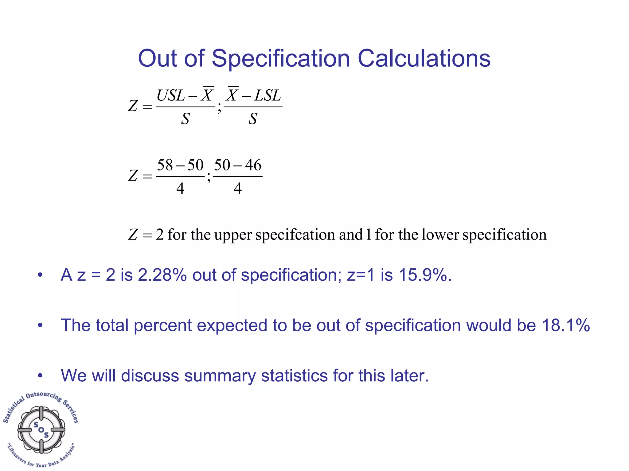
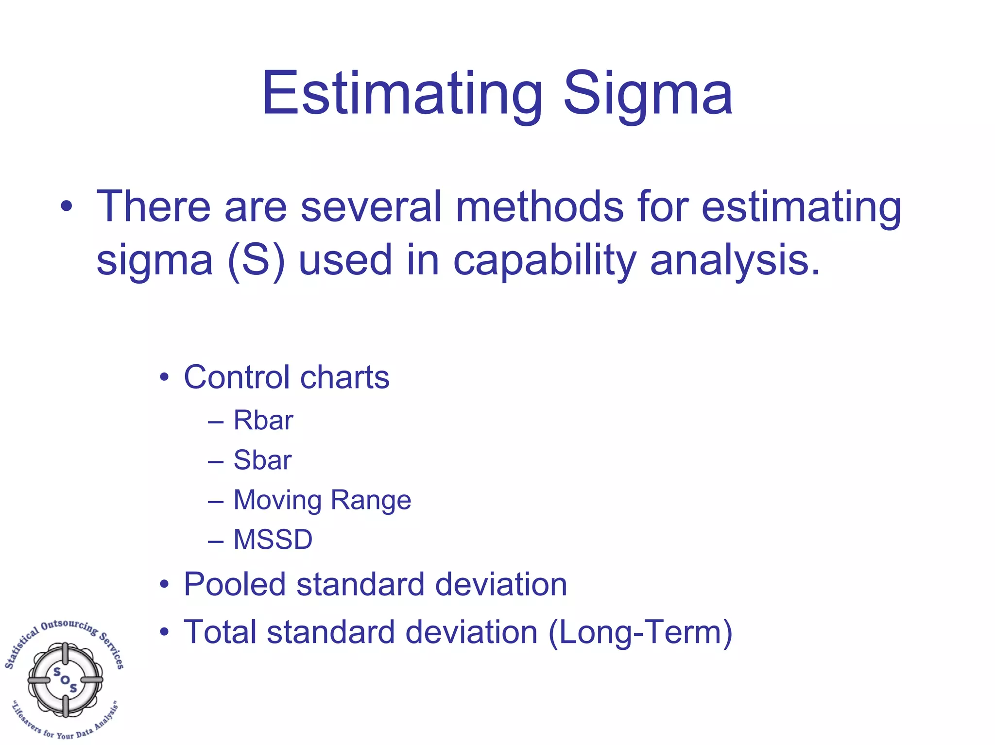
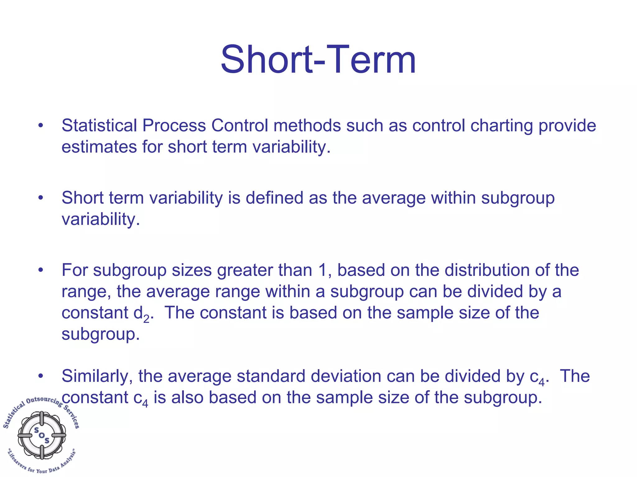
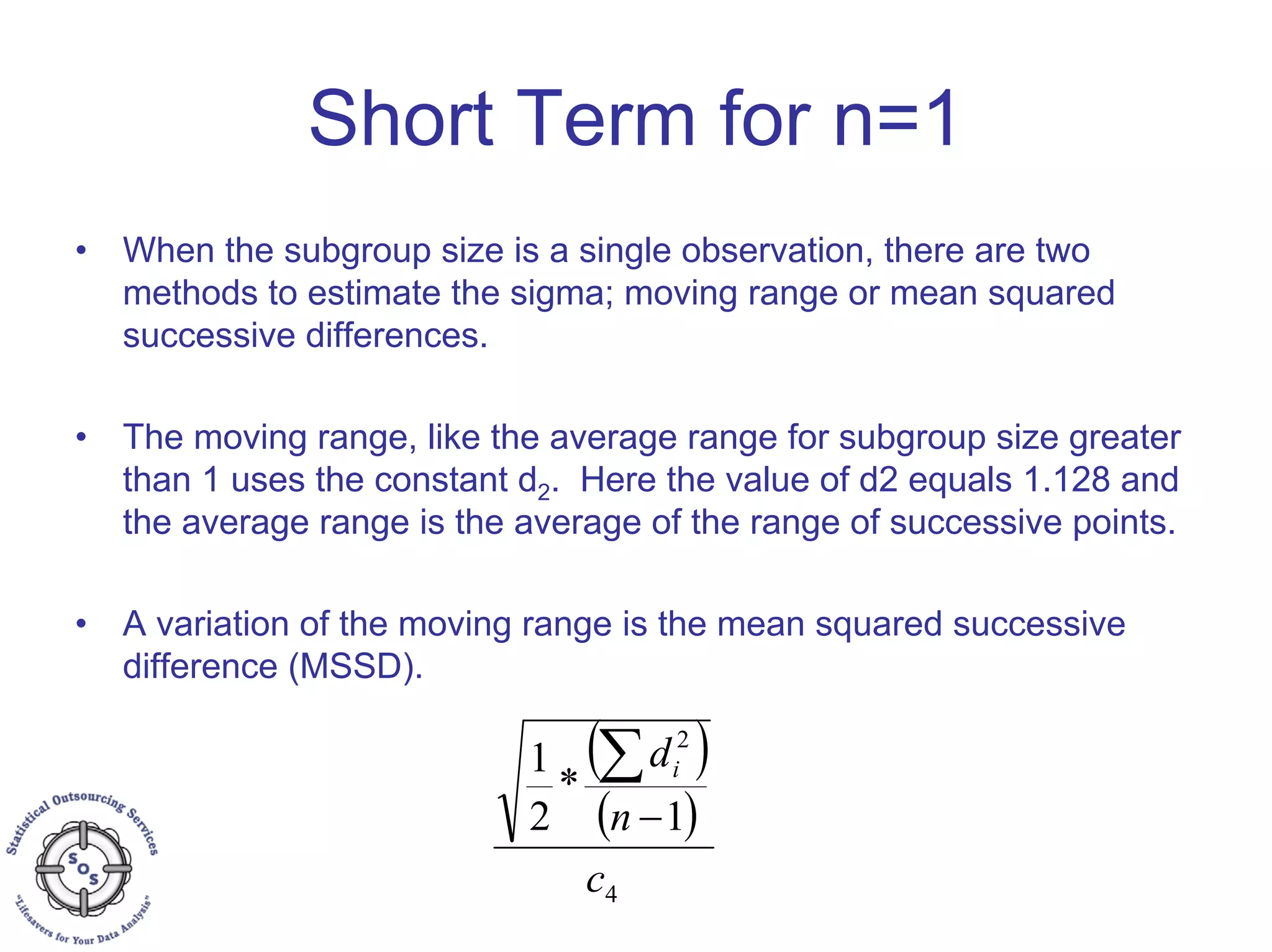
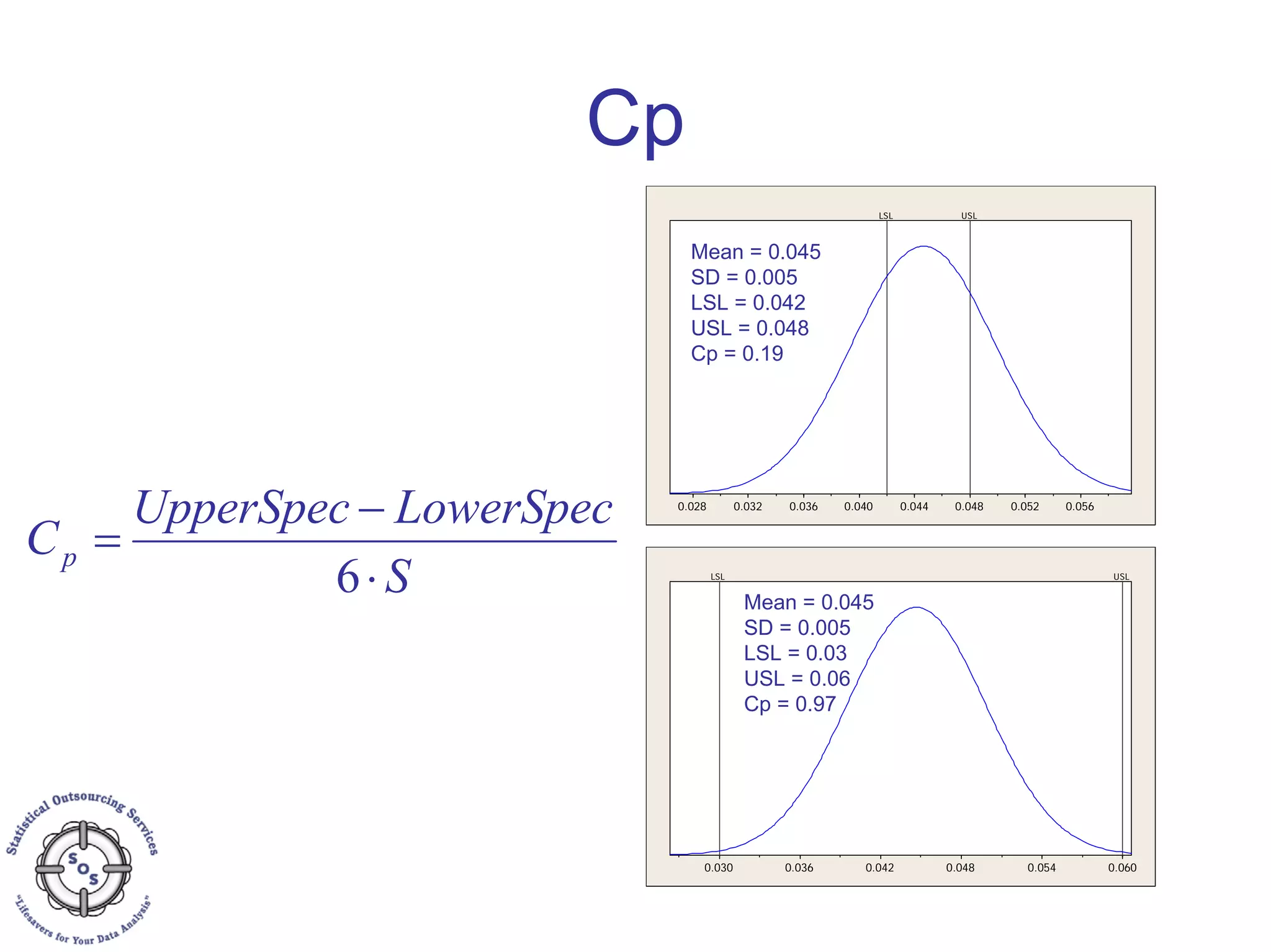
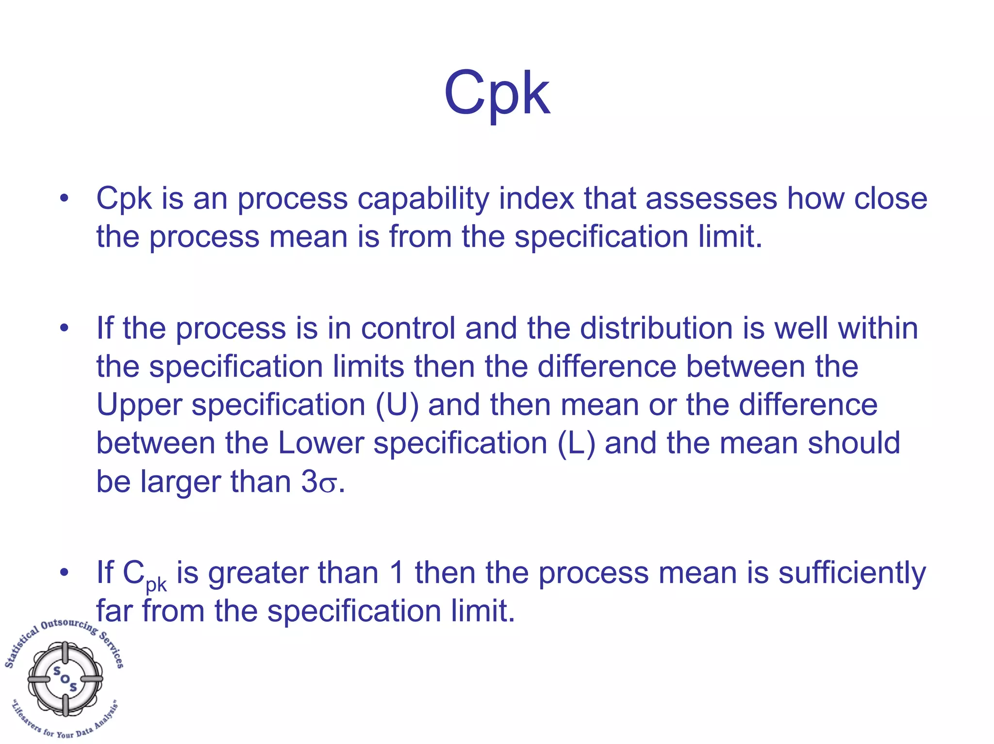
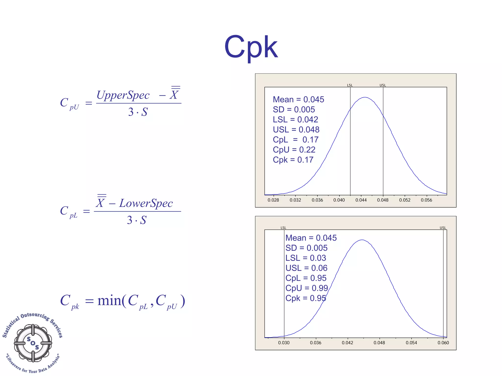
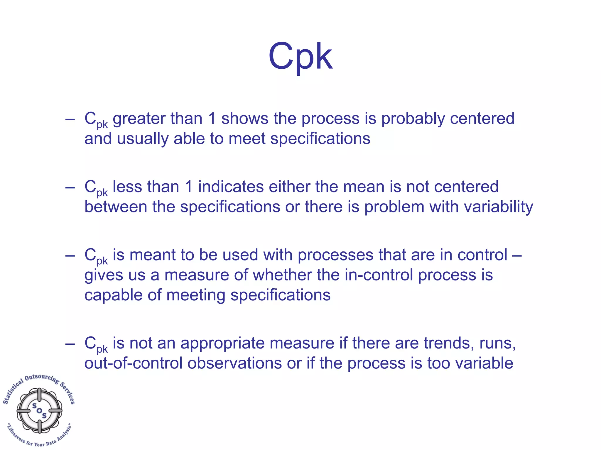
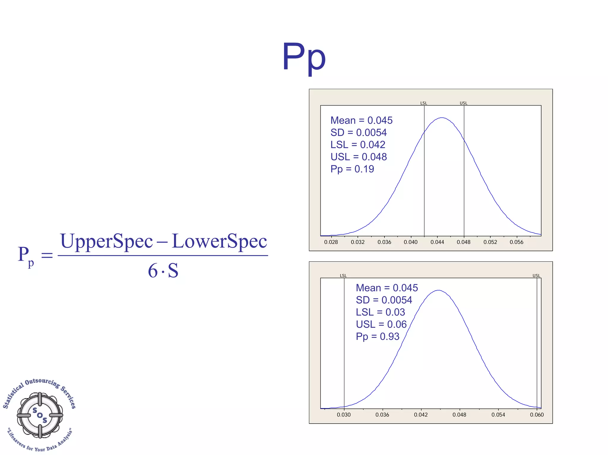
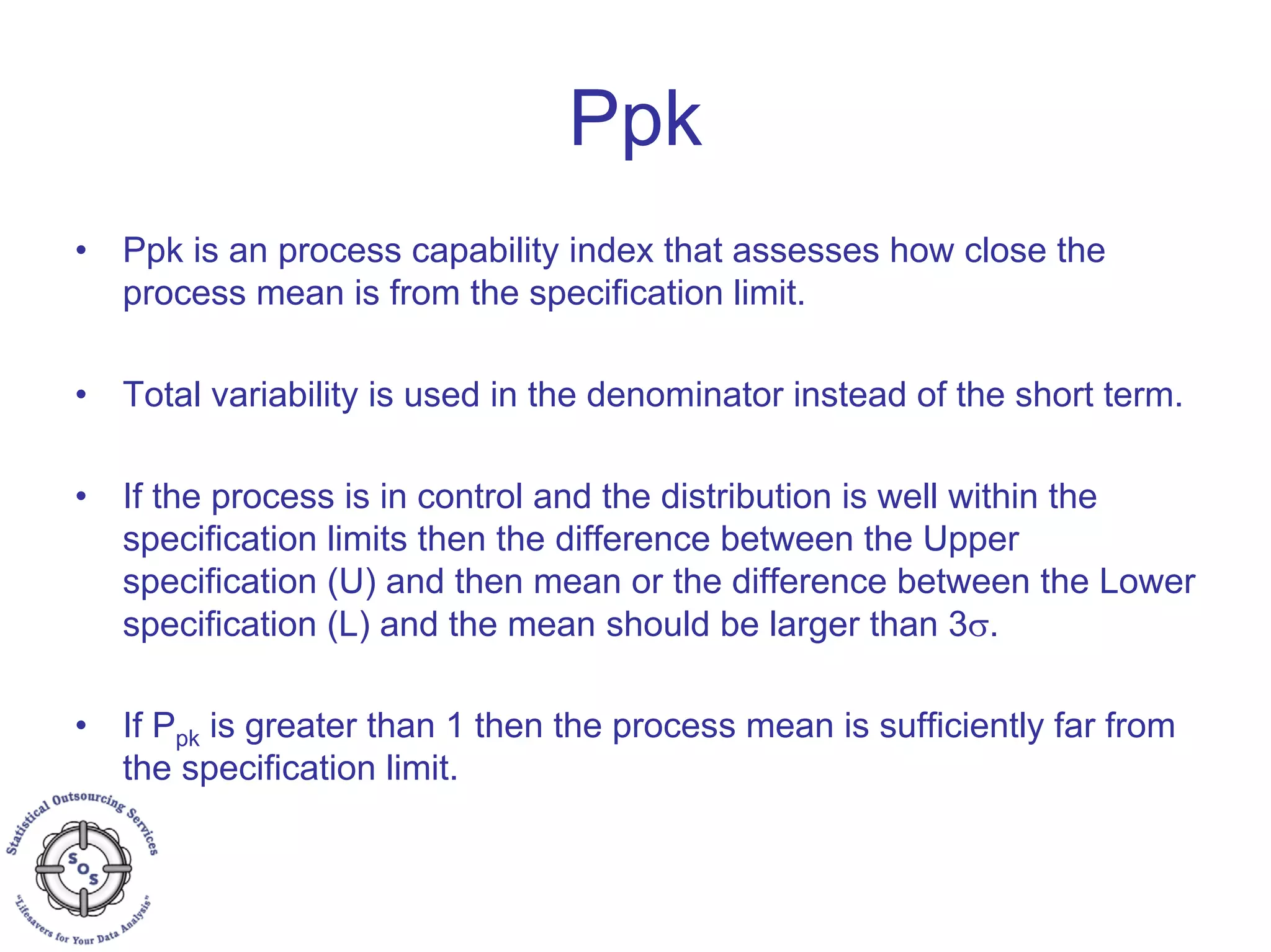
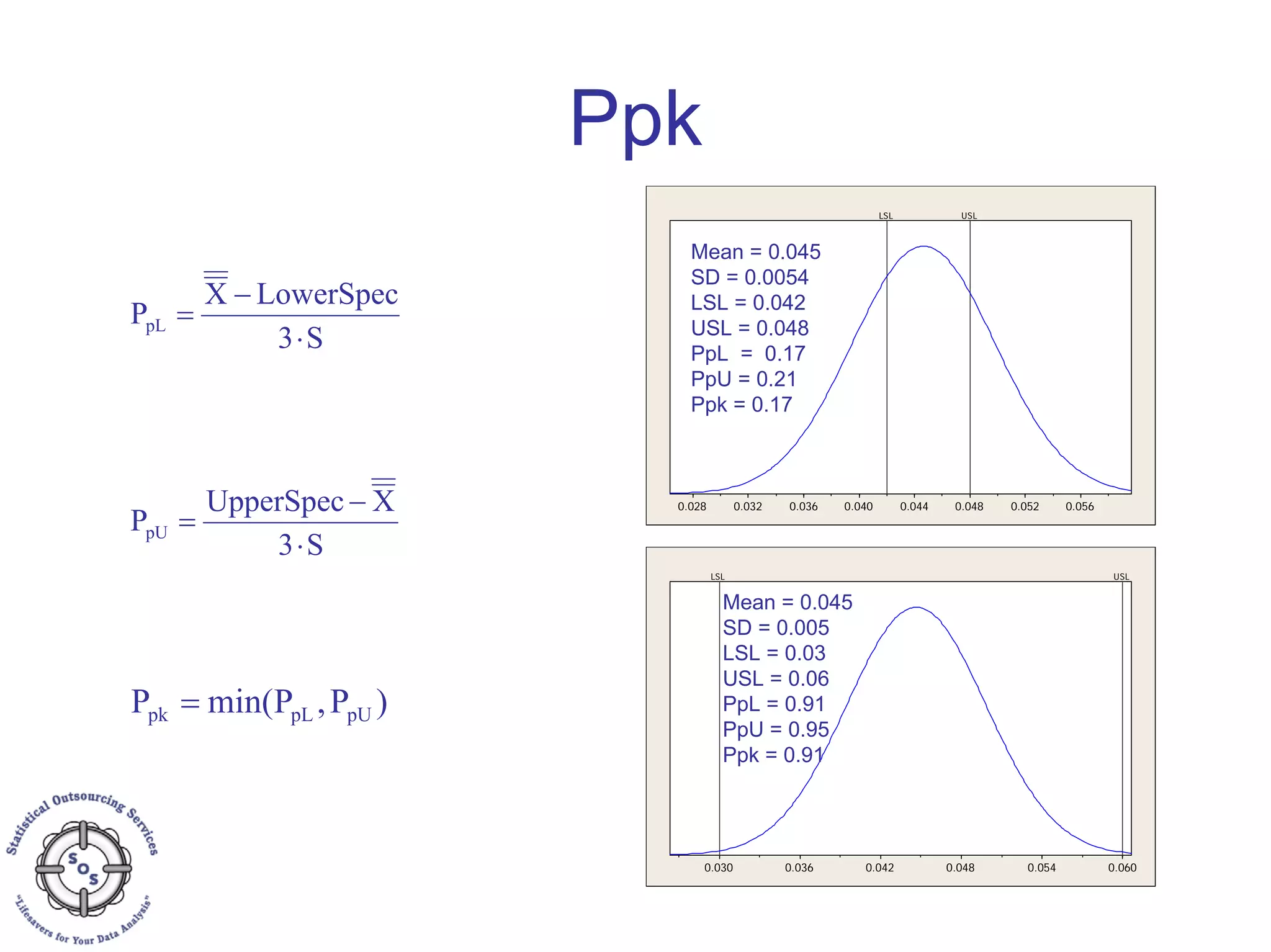
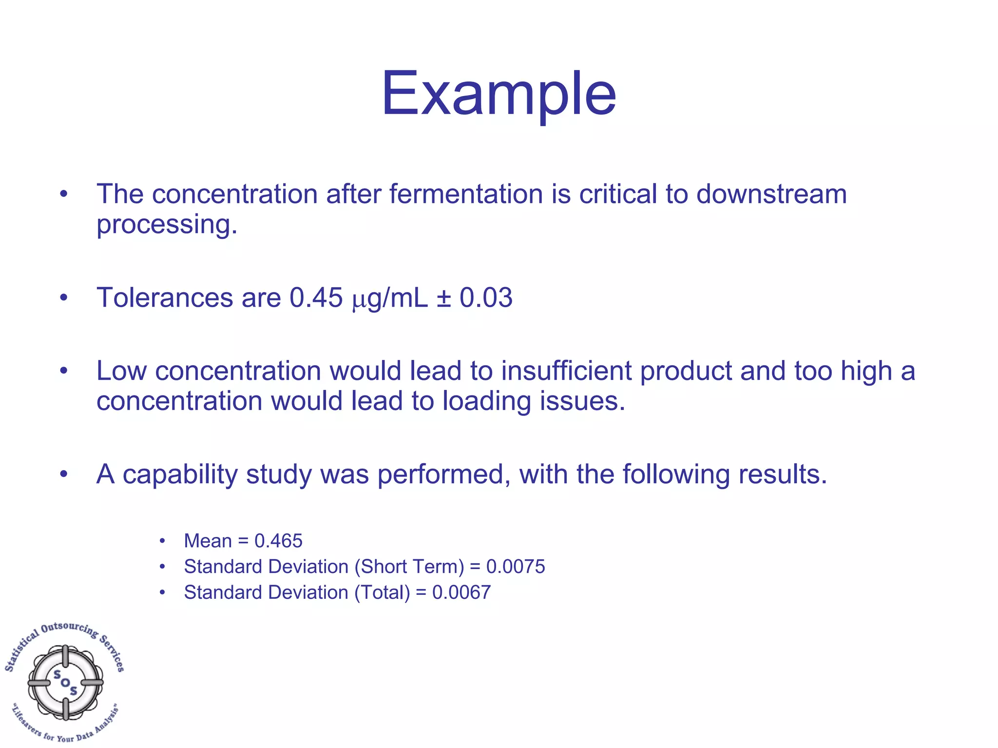
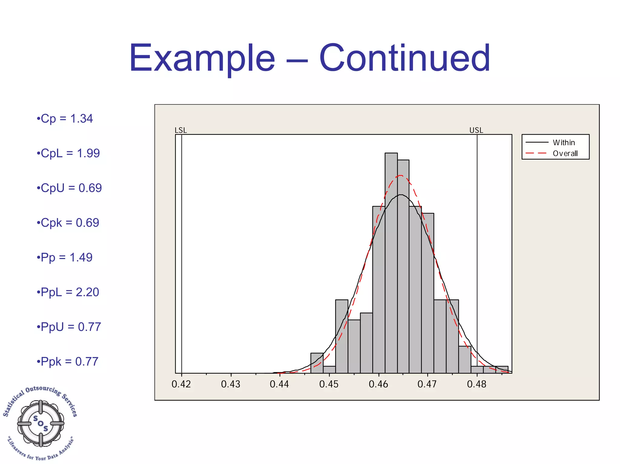
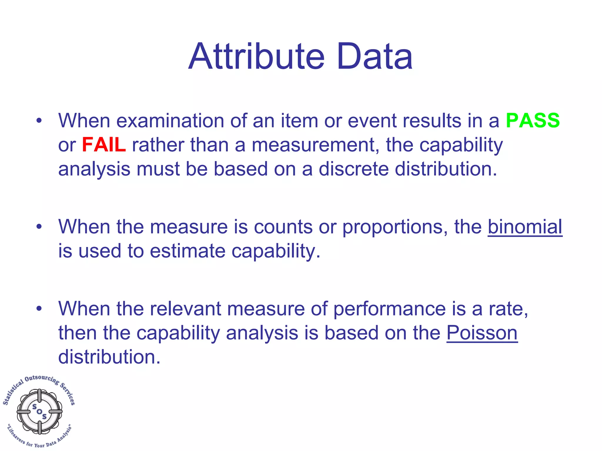
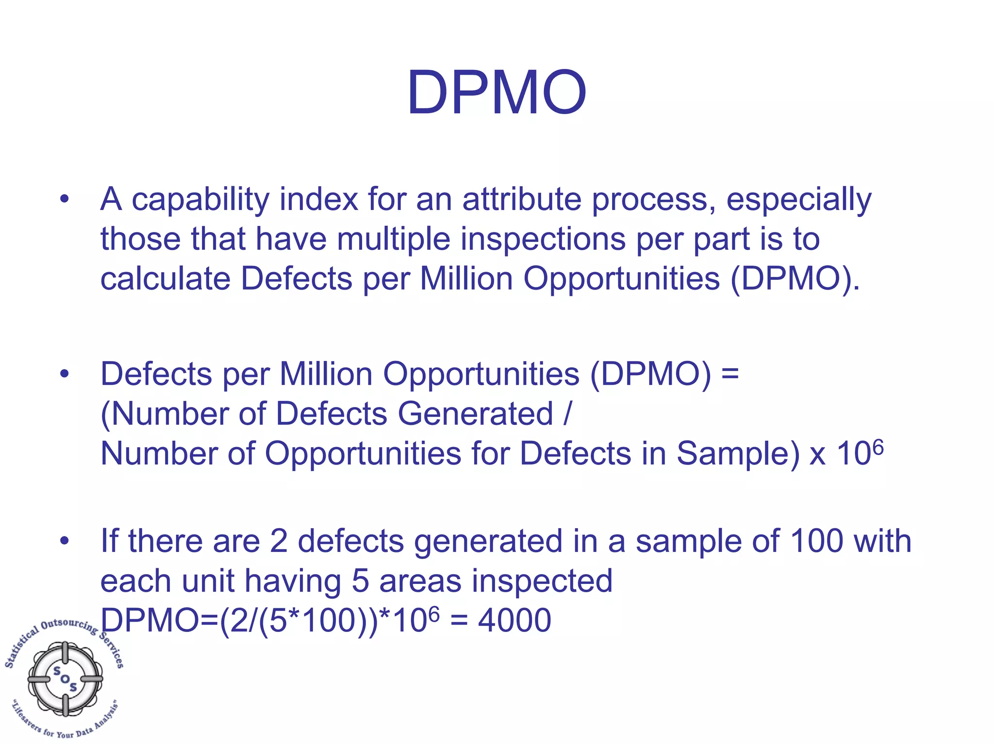
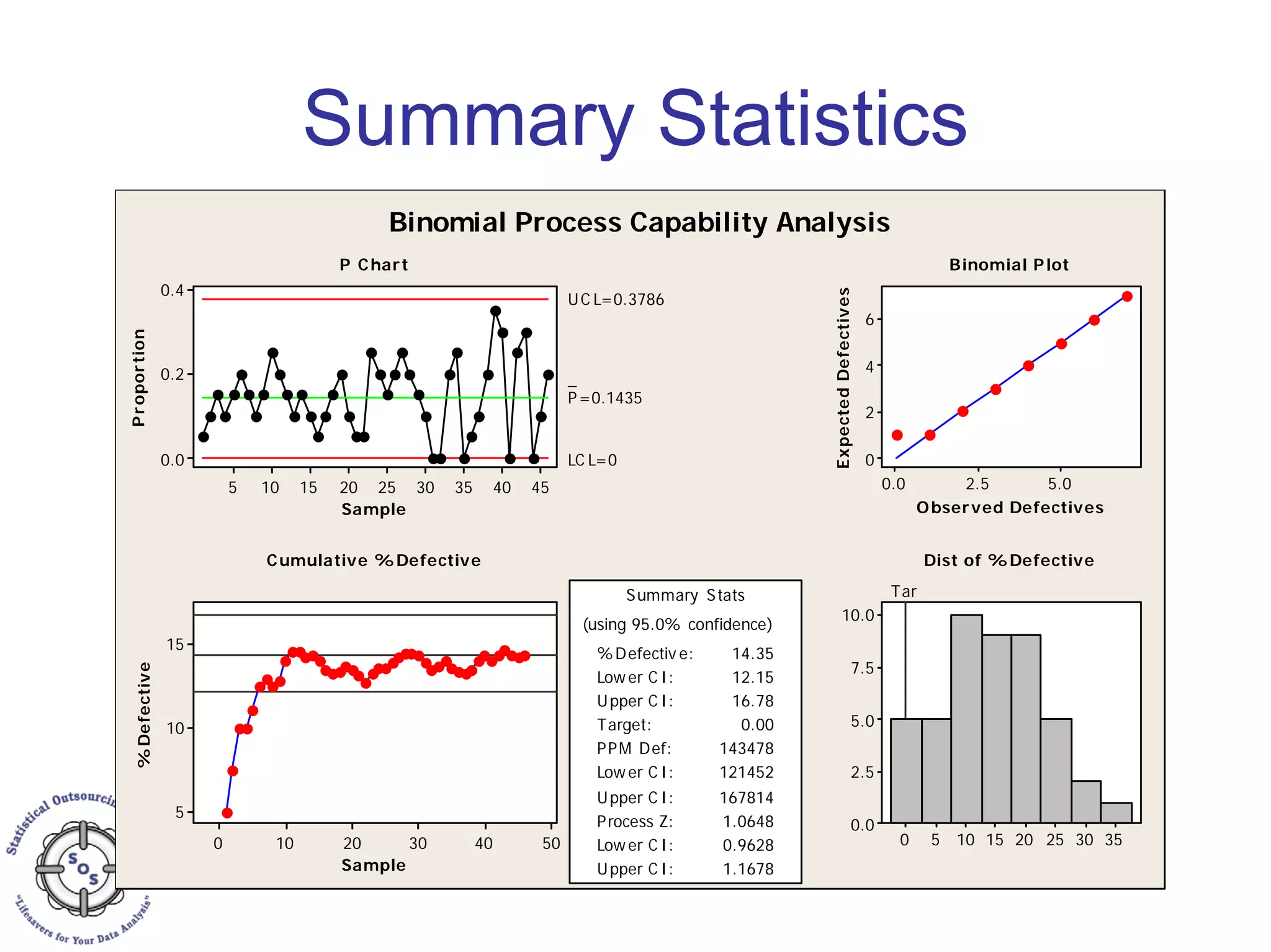
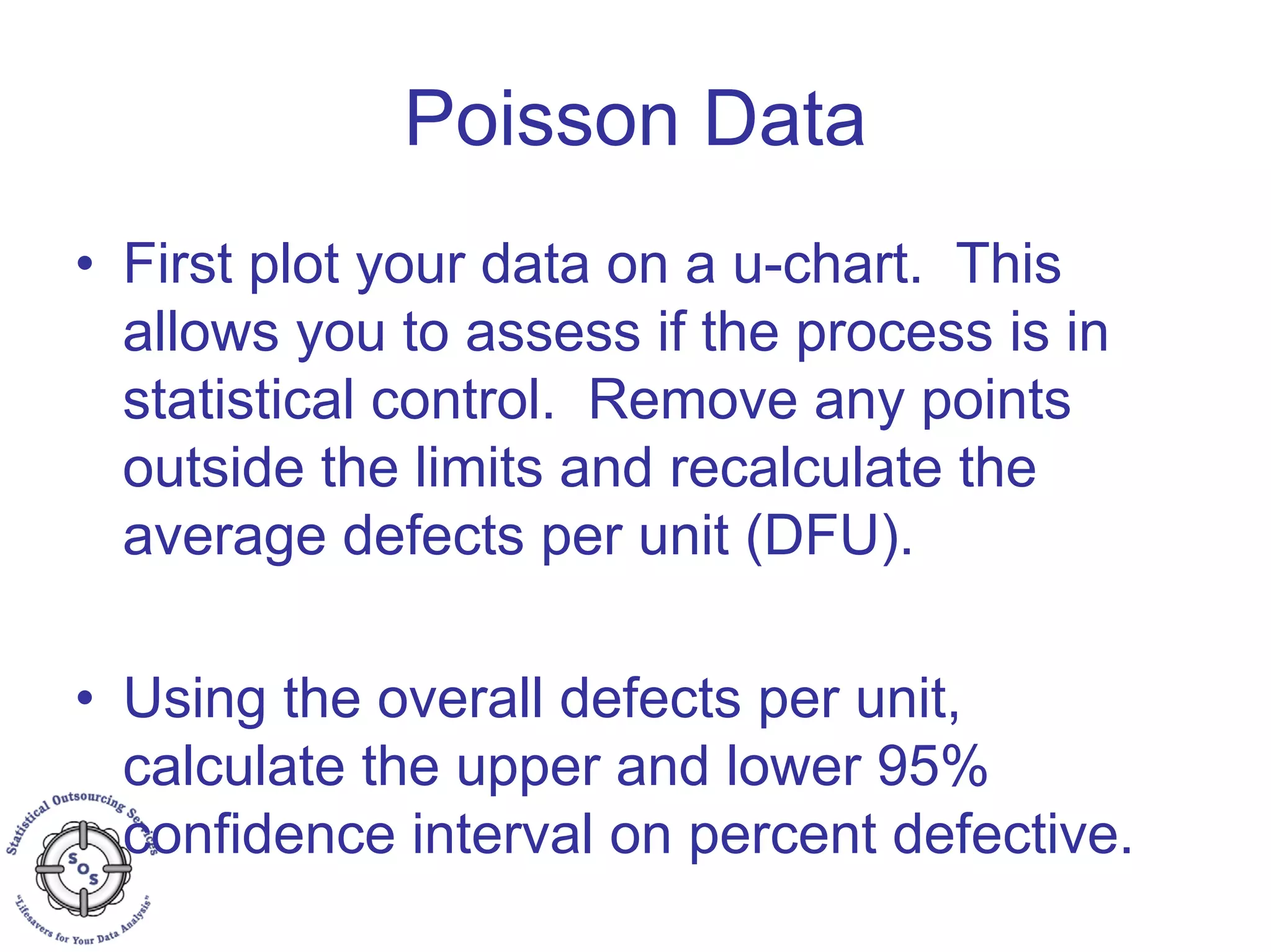
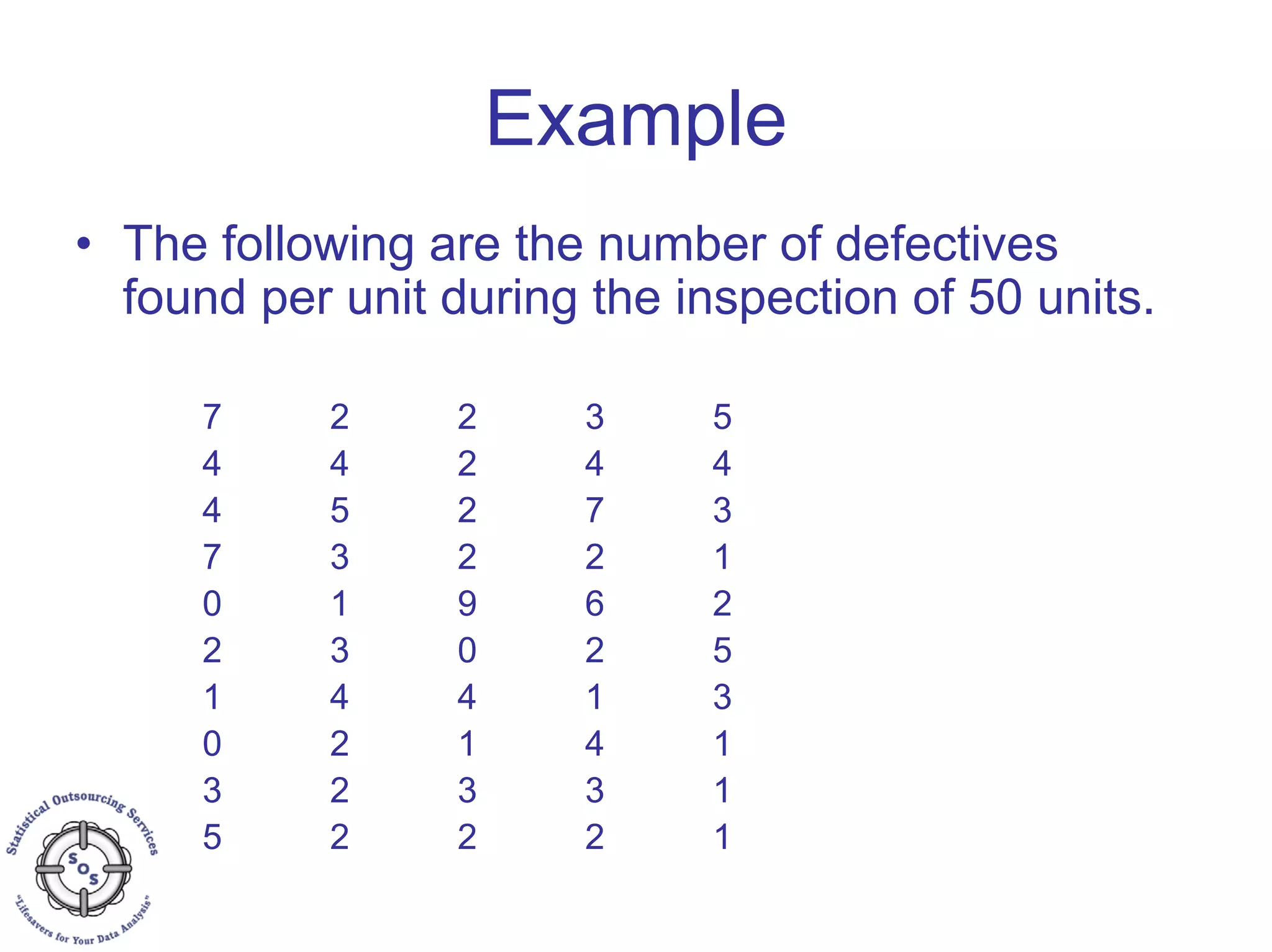
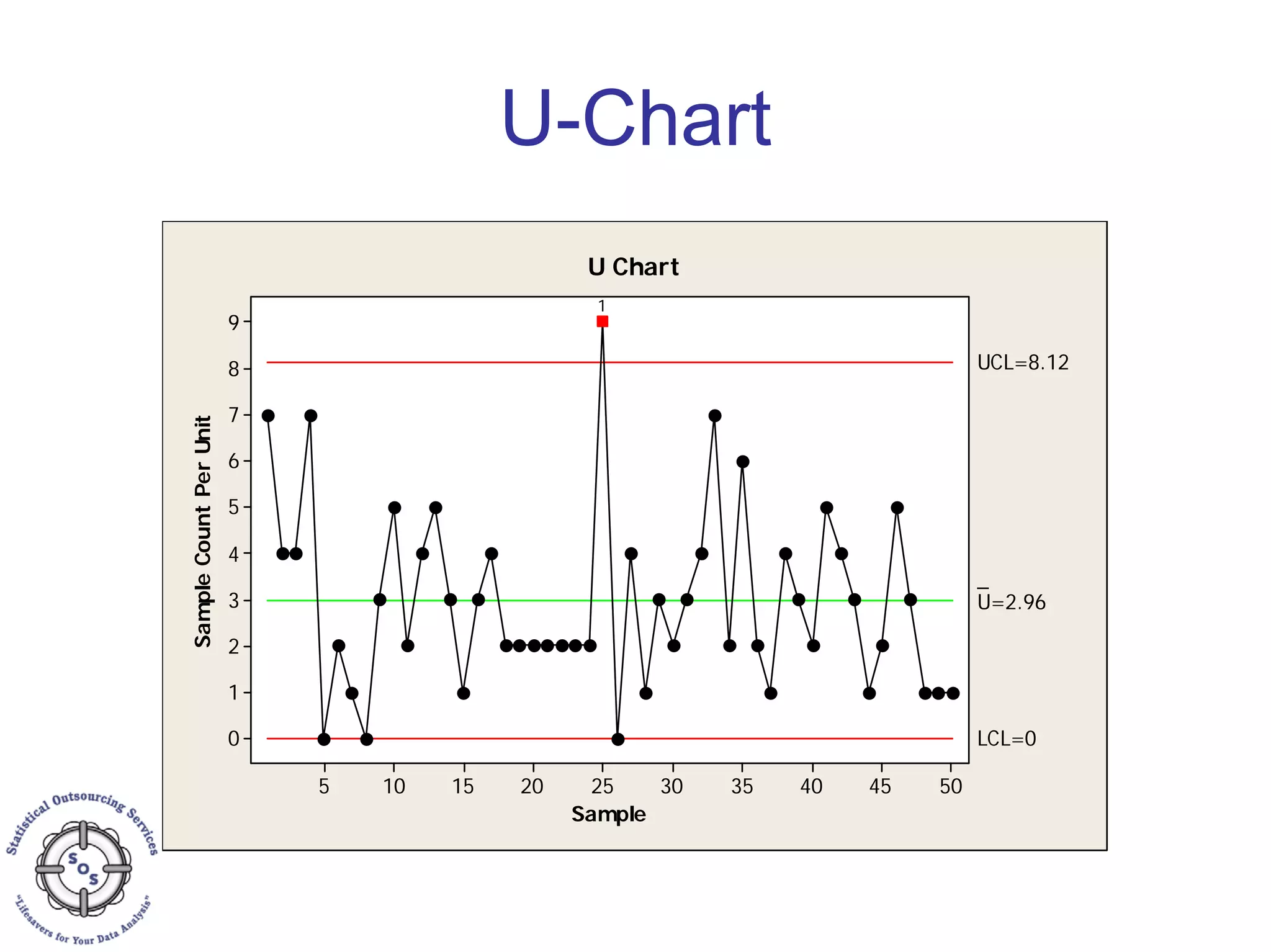
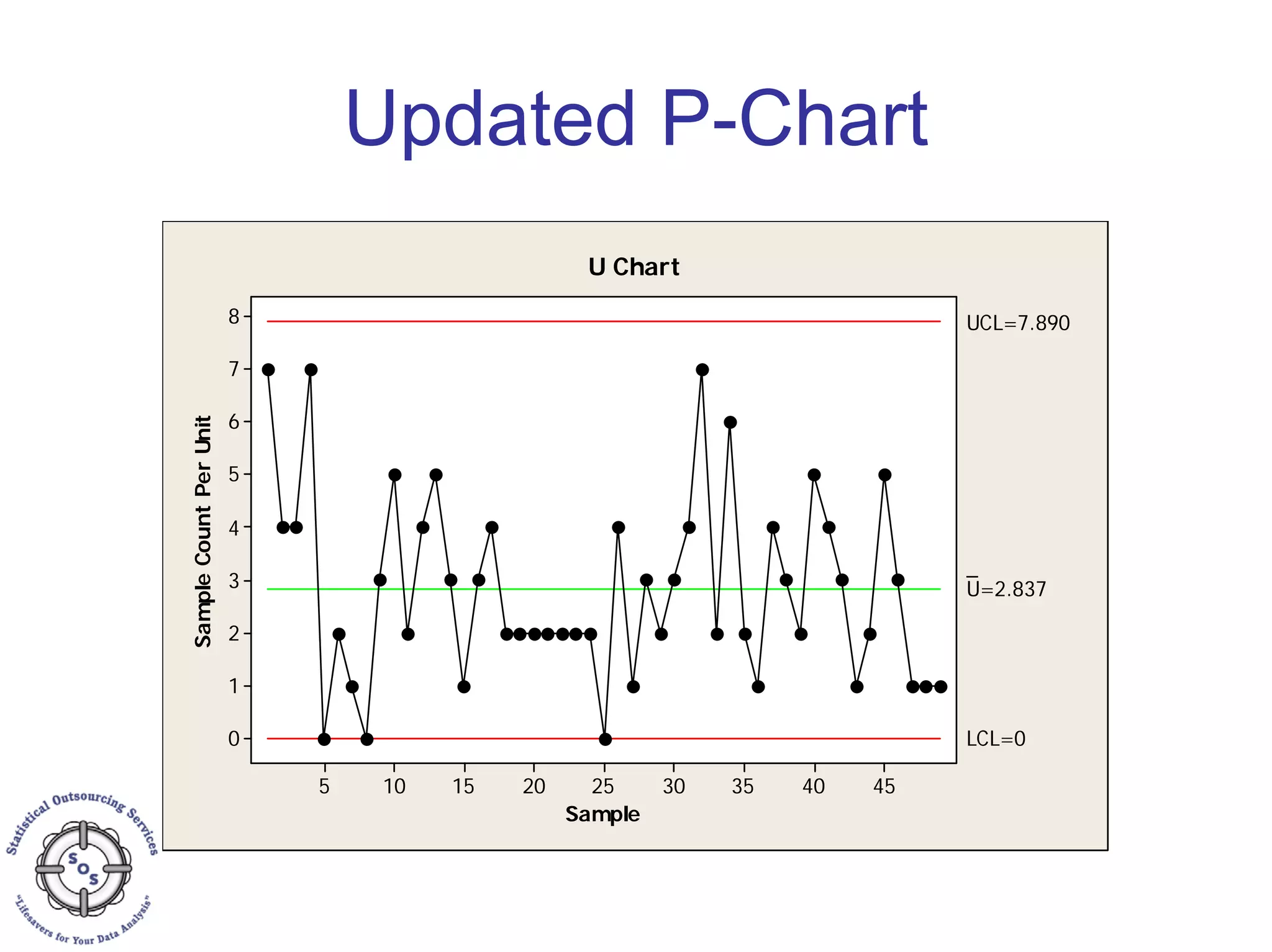
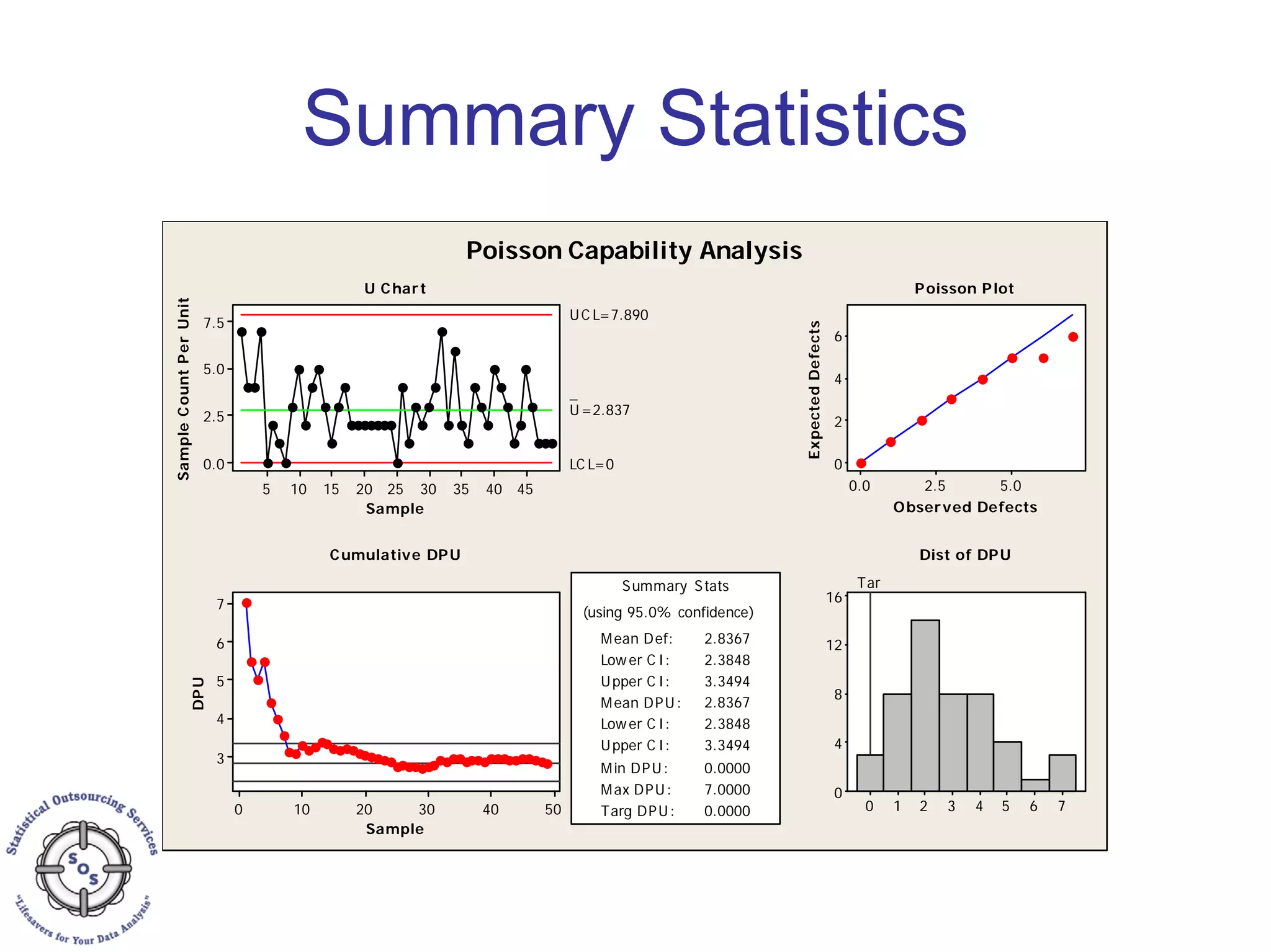
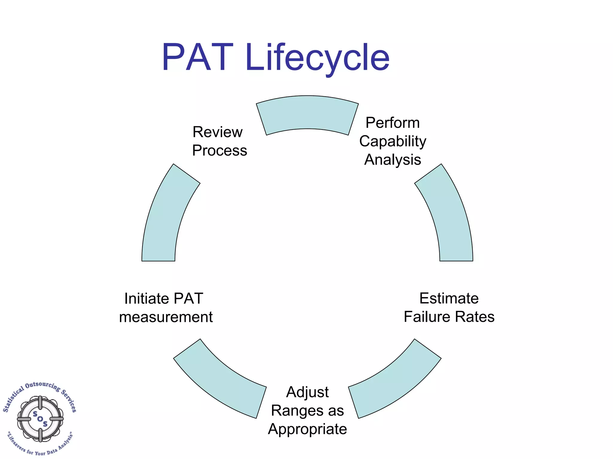
This document discusses process capability analysis and process analytical technology. It begins with an introduction to capability, including histograms and the normal distribution. It then covers capability indices like Cp, Cpk, Pp and Ppk and how to calculate sigma. It discusses using capability analysis with attribute data by calculating defects per million opportunities (DPMO). It concludes with a brief overview of process analytical technology (PAT).

1. Process Capability Analysis and Process
Analytical Technology
Presented by:
Steven Walfish
President, Statistical Outsourcing Services
steven@statisticaloutsourcingservices.com
http://www.statisticaloutsourcingservices.com

2. Agenda
• Introduction to Capability
– What is capability
– Histograms
– Normal Distribution
• Capability Indices
– Cp
– Cpk
– Pp
– Ppk
• Calculating Sigma
– Relating capability to percent nonconforming
• Capability with attribute data
– Defects per Million Opportunities (DPMO)
• Process Analytical Technology (PAT)

3. What is Capability?
• Process capability compares the output of an in-control
process to the specification limits.
• The comparison is made by forming the ratio of the
spread between the process specifications (the
specification "width") to the spread of the process
values, as measured by process standard deviation.
• A capable process is one where almost all the
measurements fall inside the specification limits.

4. Graphical Representation
76.876.275.675.074.473.873.2
LSL USL
Mean = 75
SD = 0.3
USL = 73
USL = 77
6S = 1.8
6S on each side of
the mean to the
specification limit.

5. Histogram
Frequency
76.476.075.675.274.874.474.0
40
30
20
10
0
73.66 74.11 74.41 74.71 75.31 75.61 75.91 76.36
±4.5S (99.9993%)
±3S (99.7%)
±2S (95.4%)
±1S (68.3%)

6. Examples of Capability
• Some examples of where capability
analysis can be used:
• Process that is not centered
• Process with large variability
• One-sided specifications
• Setting/confirming customer specifications

7. Percent Out of Specifications
• Based on the normal distribution, the percent of product that would
fall out of specification can be calculated.
• This is best explained using an example.
• Assume we have a process with mean = 50, standard deviation = 4,
USL = 58 and LSL = 46.
• We divide this problem into two parts. First the percent out of
specification on the high end (greater than the USL) and then the
percent out on the low end (less than the LSL).

8. The Normal Distribution
• The normal distribution is:
• Z is the number of standard deviations that the specification is from
the mean.
• Normal probability tables give you the percent of the distribution that
would exceed the specification limit for a given z value
• Remember that 68.3% of the data is within ±1S (therefore 31.7% is
outside of ±1S).
S
LSLX
S
XUSL
Z
−−
= ;

9. Out of Specification Calculations
• A z = 2 is 2.28% out of specification; z=1 is 15.9%.
• The total percent expected to be out of specification would be 18.1%
• We will discuss summary statistics for this later.
ionspecificatlowerfor the1andonspecifcatiupperfor the2
4
4650
;
4
5058
;
=
−−
=
−−
=
Z
Z
S
LSLX
S
XUSL
Z

10. Estimating Sigma
• There are several methods for estimating
sigma (S) used in capability analysis.
• Control charts
– Rbar
– Sbar
– Moving Range
– MSSD
• Pooled standard deviation
• Total standard deviation (Long-Term)

11. Short-Term
• Statistical Process Control methods such as control charting provide
estimates for short term variability.
• Short term variability is defined as the average within subgroup
variability.
• For subgroup sizes greater than 1, based on the distribution of the
range, the average range within a subgroup can be divided by a
constant d2. The constant is based on the sample size of the
subgroup.
• Similarly, the average standard deviation can be divided by c4. The
constant c4 is also based on the sample size of the subgroup.

12. Short Term for n=1
• When the subgroup size is a single observation, there are two
methods to estimate the sigma; moving range or mean squared
successive differences.
• The moving range, like the average range for subgroup size greater
than 1 uses the constant d2. Here the value of d2 equals 1.128 and
the average range is the average of the range of successive points.
• A variation of the moving range is the mean squared successive
difference (MSSD).
( )
( )
4
2
1
*
2
1
c
n
di
−
∑

13. • Total variability can be estimated from the entire data set.
• Total variability is estimated by treating the data as one big
sample using only the overall mean and looking at how the data
points vary around this one overall mean.
• Total variability estimates the long term state of the process
variability.
• If a process is stable, then the variability seen short term is
consistent with what you expect to see long term.
Long Term

14. Assumptions
• There are two critical assumptions to consider when performing
process capability analyses with continuous data, namely:
• The process is in statistical control.
• The distribution of the process considered is Normal.
• If these assumptions are not met, the resulting statistics may be
highly unreliable.
• In a later modules we will discuss capability analysis for non-normal
data.

15. Capability Indices
• There are several statistics that can be used to measure the
capability of a process: Cp, Cpk, Pp and Ppk.
• The statistics assume that the population of data values is normally
distributed.
• Variability can be stated as either short-term or long-term.
• Cp and Cpk are based on short term variability
• Pp and Ppk are based on total variability

16. Cp
• Approximately 99.7% of the data from a normal distribution is
contained between ±3σ.
• If the process is in control and the distribution is well within the
specification limits then the difference between the Upper
specification (U) and Lower specification (L) should be larger
than 6σ.
• If the specifications are larger than 6σ, the ratio will be less than 1.
• If Cp is greater than 1 then the process has the potential to meet
specifications as long as the mean is centered.

17. Cp
S
LowerSpecUpperSpec
Cp
⋅
−
=
6
0.0560.0520.0480.0440.0400.0360.0320.028
LSL USL
0.0600.0540.0480.0420.0360.030
LSL USL
Mean = 0.045
SD = 0.005
LSL = 0.042
USL = 0.048
Cp = 0.19
Mean = 0.045
SD = 0.005
LSL = 0.03
USL = 0.06
Cp = 0.97

18. Cpk
• Cpk is an process capability index that assesses how close
the process mean is from the specification limit.
• If the process is in control and the distribution is well within
the specification limits then the difference between the
Upper specification (U) and then mean or the difference
between the Lower specification (L) and the mean should
be larger than 3σ.
• If Cpk is greater than 1 then the process mean is sufficiently
far from the specification limit.

19. Cpk
0.0560.0520.0480.0440.0400.0360.0320.028
LSL USL
0.0600.0540.0480.0420.0360.030
LSL USL
Mean = 0.045
SD = 0.005
LSL = 0.042
USL = 0.048
CpL = 0.17
CpU = 0.22
Cpk = 0.17
Mean = 0.045
SD = 0.005
LSL = 0.03
USL = 0.06
CpL = 0.95
CpU = 0.99
Cpk = 0.95
S
LowerSpecX
C pL
⋅
−
=
3
S
XUpperSpec
C pU
⋅
−
=
3
),min( pUpLpk
CCC =

20. – Cpk greater than 1 shows the process is probably centered
and usually able to meet specifications
– Cpk less than 1 indicates either the mean is not centered
between the specifications or there is problem with variability
– Cpk is meant to be used with processes that are in control –
gives us a measure of whether the in-control process is
capable of meeting specifications
– Cpk is not an appropriate measure if there are trends, runs,
out-of-control observations or if the process is too variable
Cpk

21. Pp
• Pp is an overall capability similar to Cp.
• Total variability is used in the denominator instead of the
short term.
• If the process is stable and in control the estimate of Pp is
similar to the estimate of Cp.
• If Pp is greater than 1 then the process is meeting the
specifications as long as the mean is centered.

22. Pp
0.0560.0520.0480.0440.0400.0360.0320.028
LSL USL
0.0600.0540.0480.0420.0360.030
LSL USL
Mean = 0.045
SD = 0.0054
LSL = 0.042
USL = 0.048
Pp = 0.19
Mean = 0.045
SD = 0.0054
LSL = 0.03
USL = 0.06
Pp = 0.93
S6
LowerSpecUpperSpec
Pp
⋅
−
=

23. Ppk
• Ppk is an process capability index that assesses how close the
process mean is from the specification limit.
• Total variability is used in the denominator instead of the short term.
• If the process is in control and the distribution is well within the
specification limits then the difference between the Upper
specification (U) and then mean or the difference between the Lower
specification (L) and the mean should be larger than 3σ.
• If Ppk is greater than 1 then the process mean is sufficiently far from
the specification limit.

24. Ppk
0.0560.0520.0480.0440.0400.0360.0320.028
LSL USL
0.0600.0540.0480.0420.0360.030
LSL USL
Mean = 0.045
SD = 0.0054
LSL = 0.042
USL = 0.048
PpL = 0.17
PpU = 0.21
Ppk = 0.17
Mean = 0.045
SD = 0.005
LSL = 0.03
USL = 0.06
PpL = 0.91
PpU = 0.95
Ppk = 0.91
)P,Pmin(P pUpLpk =
S3
LowerSpecX
PpL
⋅
−
=
S3
XUpperSpec
PpU
⋅
−
=

25. Example
• The concentration after fermentation is critical to downstream
processing.
• Tolerances are 0.45 μg/mL ± 0.03
• Low concentration would lead to insufficient product and too high a
concentration would lead to loading issues.
• A capability study was performed, with the following results.
• Mean = 0.465
• Standard Deviation (Short Term) = 0.0075
• Standard Deviation (Total) = 0.0067

26. Example – Continued
•Cp = 1.34
•CpL = 1.99
•CpU = 0.69
•Cpk = 0.69
•Pp = 1.49
•PpL = 2.20
•PpU = 0.77
•Ppk = 0.77
0.480.470.460.450.440.430.42
LSL USL
Within
Overall

27. Attribute Data
• When examination of an item or event results in a PASS
or FAIL rather than a measurement, the capability
analysis must be based on a discrete distribution.
• When the measure is counts or proportions, the binomial
is used to estimate capability.
• When the relevant measure of performance is a rate,
then the capability analysis is based on the Poisson
distribution.

28. DPMO
• A capability index for an attribute process, especially
those that have multiple inspections per part is to
calculate Defects per Million Opportunities (DPMO).
• Defects per Million Opportunities (DPMO) =
(Number of Defects Generated /
Number of Opportunities for Defects in Sample) x 106
• If there are 2 defects generated in a sample of 100 with
each unit having 5 areas inspected
DPMO=(2/(5*100))*106 = 4000

29. Binomial Data
• First plot your data on a p-chart. This allows you to assess if the
process is in statistical control. Remove any points outside the limits
and recalculate the average percent defective.
• Using the overall percent defective, calculate the upper and lower
95% confidence interval on percent defective.
• Multiply the percent defective by 1,000,000 to get the DPMO.
• Calculate Process Z by determining the Z-value that corresponds to
the percent defective. A higher Process Z is desirable.

30. Example
• The following are the number of defectives
found during the inspection of 20 units in each
lot.
1 4 1 2 4
2 3 1 0 7
3 2 5 8 8
2 3 4 9 6
3 2 3 0 0
4 1 4 4 5
3 2 5 5 6
2 3 9 0 0
3 4 4 1 2
5 2 3 2 4

31. P-Chart
Sample
Proportion
5045403530252015105
0.5
0.4
0.3
0.2
0.1
0.0
_
P=0.166
UCL=0.4156
LCL=0
11
P Chart

32. Updated P-Chart
Sample
Proportion
45403530252015105
0.4
0.3
0.2
0.1
0.0
_
P=0.1435
UCL=0.3786
LCL=0
P Chart

33. Summary Statistics
Sample
Proportion
45403530252015105
0.4
0.2
0.0
_
P=0.1435
UC L=0.3786
LC L=0
Sample
%Defective
50403020100
15
10
5
Summary Stats
0.00
PPM Def: 143478
Low er C I: 121452
Upper C I: 167814
Process Z: 1.0648
Lower C I:
(using 95.0% confidence)
0.9628
Upper C I: 1.1678
%Defectiv e: 14.35
Low er C I: 12.15
Upper C I: 16.78
Target:
Observed Defectives
ExpectedDefectives
5.02.50.0
6
4
2
0
35302520151050
10.0
7.5
5.0
2.5
0.0
Tar
Binomial Process Capability Analysis
P Chart
Cumulative %Defective
Binomial Plot
Dist of %Defective

34. Poisson Data
• First plot your data on a u-chart. This
allows you to assess if the process is in
statistical control. Remove any points
outside the limits and recalculate the
average defects per unit (DFU).
• Using the overall defects per unit,
calculate the upper and lower 95%
confidence interval on percent defective.

35. Example
• The following are the number of defectives
found per unit during the inspection of 50 units.
7 2 2 3 5
4 4 2 4 4
4 5 2 7 3
7 3 2 2 1
0 1 9 6 2
2 3 0 2 5
1 4 4 1 3
0 2 1 4 1
3 2 3 3 1
5 2 2 2 1

36. U-Chart
Sample
SampleCountPerUnit
5045403530252015105
9
8
7
6
5
4
3
2
1
0
_
U=2.96
UCL=8.12
LCL=0
1
U Chart

37. Updated P-Chart
Sample
SampleCountPerUnit
45403530252015105
8
7
6
5
4
3
2
1
0
_
U=2.837
UCL=7.890
LCL=0
U Chart

38. Summary Statistics
Sample
SampleCountPerUnit
45403530252015105
7.5
5.0
2.5
0.0
_
U=2.837
UC L=7.890
LC L=0
Sample
DPU
50403020100
7
6
5
4
3
Summary Stats
2.8367
Lower C I: 2.3848
Upper C I: 3.3494
Min DPU: 0.0000
Max DPU: 7.0000
Targ DPU:
(using 95.0% confidence)
0.0000
Mean Def: 2.8367
Lower C I: 2.3848
Upper C I: 3.3494
Mean DPU:
Observed Defects
ExpectedDefects
5.02.50.0
6
4
2
0
76543210
16
12
8
4
0
Tar
Poisson Capability Analysis
U Chart
Cumulative DPU
Poisson Plot
Dist of DPU

39. Process Analytical Technology
• The goal of PAT is to achieve sufficient
process understanding and control to
enable quality assurance in “real-time”.
• When a process is capable and
repeatable, this can be achieved.
• When there is too much variability, then
further process understanding is required.

40. PAT Lifecycle
Adjust
Ranges as
Appropriate
Estimate
Failure Rates
Perform
Capability
Analysis
Initiate PAT
measurement
Review
Process

41. Conclusions
• Process capability analysis can be predictive of
expected out of specification results.
• The process must be in statistical control prior to
doing a capability analysis.
• Data transformation can be used for non-normal
data.
• Attribute data can use confidence intervals to
predict process performance.

42. Questions?

43. Statistical Outsourcing Services
• Statistical Outsourcing Services
can provide:
– Bioassay Analysis
– Acceptance Sampling
– Method Validation
– Process Validation
– Stability Testing
– Comparability Studies
– Quality Systems
– Statistical Process Control (SPC)
– Third Party Expert Review
– Clinical Protocol Review
– Business Intelligence (BI)
• The following is a sample list of
available training programs:
– Introduction to Statistics
– Statistics for Non-Statisticians
– Using Statistical Software
– Statistical Process Control (SPC)
– Regression Analysis
– Design of Experiments
– Method Validation