The document discusses minimum spanning trees (MST) and two algorithms for finding them: Prim's algorithm and Kruskal's algorithm. It begins by defining an MST as a spanning tree (connected acyclic graph containing all vertices) with minimum total edge weight. Prim's algorithm grows a single tree by repeatedly adding the minimum weight edge connecting the growing tree to another vertex. Kruskal's algorithm grows a forest by repeatedly merging two components via the minimum weight edge connecting them. Both algorithms produce optimal MSTs by adding only "safe" edges that cannot be part of a cycle.

1. Minimum Spanning Trees (MST)

2. Minimum Spanning Trees
• Spanning Tree
– A tree (i.e., connected, acyclic graph) which contains
all the vertices of the graph
• Minimum Spanning Tree
– Spanning tree with the minimum sum of weights
• Spanning forest
– If a graph is not connected, then there is a spanning
tree for each connected component of the graph
a
b c d
e
g g f
i
4
8 7
8
11
1 2
7
2
4 14
9
10
6

3. Applications of MST
– Find the least expensive way to connect a set of
cities, terminals, computers, etc.

4. Example
Problem
• A town has a set of houses
and a set of roads
• A road connects 2 and only
2 houses
• A road connecting houses u and v has a repair
cost w(u, v)
Goal: Repair enough (and no more) roads such
that:
1. Everyone stays connected
i.e., can reach every house from all other houses
2. Total repair cost is minimum
a
b c d
e
h g f
i
4
8 7
8
11
1 2
7
2
4 14
9
10
6

5. Properties of Minimum Spanning Trees
• Minimum spanning tree is not unique
• MST has no cycles – see why:
– We can take out an edge of a cycle, and still have
the vertices connected while reducing the cost
• # of edges in a MST:
– |V| - 1

6. Growing a MST – Generic Approach
a
b c d
e
h g f
i
4
8 7
8
11
1 2
7
2
4 14
9
10
6
• Grow a set A of edges (initially
empty)
• Incrementally add edges to A
such that they would belong
to a MST
– An edge (u, v) is safe for A if and
only if A  {(u, v)} is also a subset
of some MST
Idea: add only “safe” edges

7. Generic MST algorithm
1. A ← 
2. while A is not a spanning tree
3. do find an edge (u, v) that is safe for A
4. A ← A  {(u, v)}
5. return A
• How do we find safe edges?
a
b c d
e
h g f
i
4
8 7
8
11
1 2
7
2
4 14
9
10
6

8. S
V - S
Finding Safe Edges
• Let’s look at edge (h, g)
– Is it safe for A initially?
• Later on:
– Let S  V be any set of vertices that includes h but not
g (so that g is in V - S)
– In any MST, there has to be one edge (at least) that
connects S with V - S
– Why not choose the edge with minimum weight (h,g)?
a
b c d
e
h g f
i
4
8 7
8
11
1 2
7
2
4 14
9
10
6

9. Definitions
• A cut (S, V - S)
is a partition of vertices
into disjoint sets S and V - S
• An edge crosses the cut
(S, V - S) if one endpoint is in S
and the other in V – S
a
b c d
e
h g f
i
4
8 7
8
11
1 2
7
2
4 14
9
10
6
S
V- S 
S
 V- S

10. Definitions (cont’d)
• A cut respects a set A
of edges  no edge
in A crosses the cut
• An edge is a light edge
crossing a cut  its weight is minimum over all
edges crossing the cut
– Note that for a given cut, there can be > 1 light
edges crossing it
a
b c d
e
h g f
i
4
8 7
8
11
1 2
7
2
4 14
9
10
6
S
V- S 
S
 V- S

11. Prim’s Algorithm
• The edges in set A always form a single tree
• Starts from an arbitrary “root”: VA = {a}
• At each step:
– Find a light edge crossing (VA, V - VA)
– Add this edge to A
– Repeat until the tree spans all vertices
a
b c d
e
h g f
i
4
8 7
8
11
1 2
7
2
4 14
9
10
6

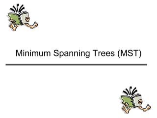
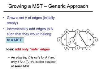
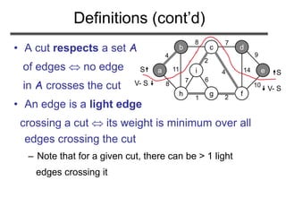
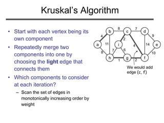
12. How to Find Light Edges Quickly?
Use a priority queue Q:
• Contains vertices not yet
included in the tree, i.e., (V – VA)
– VA = {a}, Q = {b, c, d, e, f, g, h, i}
• We associate a key with each vertex v:
key[v] = minimum weight of any edge (u, v)
connecting v to VA
a
b c d
e
h g f
i
4
8 7
8
11
1 2
7
2
4 14
9
10
6
w1
w2
Key[a]=min(w1,w2)
a

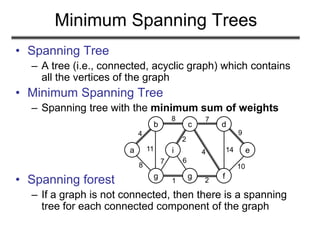
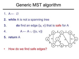
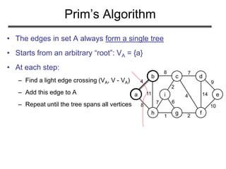
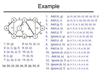
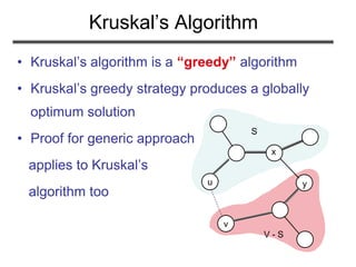
13. How to Find Light Edges Quickly?
(cont.)
• After adding a new node to VA we update the weights of all
the nodes adjacent to it
e.g., after adding a to the tree, k[b]=4 and k[h]=8
• Key of v is  if v is not adjacent to any vertices in VA
a
b c d
e
h g f
i
4
8 7
8
11
1 2
7
2
4 14
9
10
6

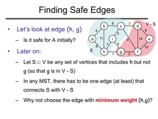
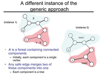
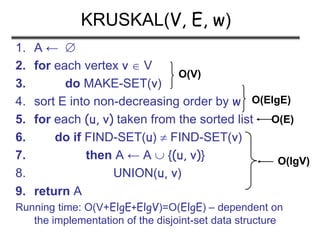
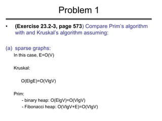
14. Example
0        
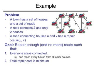
Q = {a, b, c, d, e, f, g, h, i}
VA = 
Extract-MIN(Q)  a
a
b c d
e
h g f
i
4
8 7
8
11
1 2
7
2
4 14
9
10
6
a
b c d
e
h g f
i
4
8 7
8
11
1 2
7
2
4 14
9
10
6
key [b] = 4  [b] = a
key [h] = 8  [h] = a
4      8 
Q = {b, c, d, e, f, g, h, i} VA = {a}
Extract-MIN(Q)  b
  
 
  
 
 
 
4
8

15. 4 

8  
8

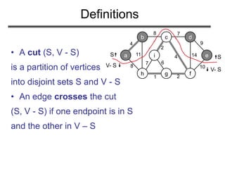
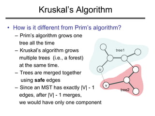
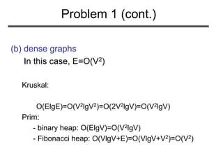
Example
a
b c d
e
h g f
i
4
8 7
8
11
1 2
7
2
4 14
9
10
6
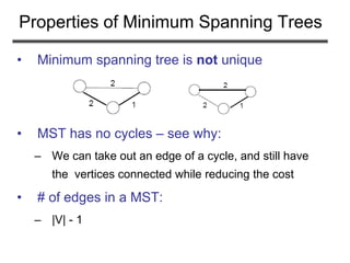
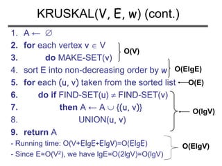
key [c] = 8  [c] = b
key [h] = 8  [h] = a - unchanged
8     8 
Q = {c, d, e, f, g, h, i} VA = {a, b}
Extract-MIN(Q)  c
a
b c d
e
h g f
i
4
8 7
8
11
1 2
7
2
4 14
9
10
6
key [d] = 7  [d] = c
key [f] = 4  [f] = c
key [i] = 2  [i] = c
7  4  8 2
Q = {d, e, f, g, h, i} VA = {a, b, c}
Extract-MIN(Q)  i


4 

8  
8
7
4
2

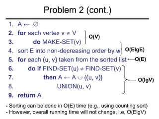
16. Example
a
b c d
e
h g f
i
4
8 7
8
11
1 2
7
2
4 14
9
10
6
key [h] = 7  [h] = i
key [g] = 6  [g] = i
7  4 6 8
Q = {d, e, f, g, h} VA = {a, b, c, i}
Extract-MIN(Q)  f
a
b c d
e
h g f
i
4
8 7
8
11
1 2
7
2
4 14
9
10
6
key [g] = 2  [g] = f
key [d] = 7  [d] = c unchanged
key [e] = 10  [e] = f
7 10 2 8
Q = {d, e, g, h} VA = {a, b, c, i, f}
Extract-MIN(Q)  g
4 7

8  4
8
2
7 6
4 7

7 6 4
8
2
2
10

17. Example
a
b c d
e
h g f
i
4
8 7
8
11
1 2
7
2
4 14
9
10
6
key [h] = 1  [h] = g
7 10 1
Q = {d, e, h} VA = {a, b, c, i, f, g}
Extract-MIN(Q)  h
a
b c d
e
h g f
i
4
8 7
8
11
1 2
7
2
4 14
9
10
6
7 10
Q = {d, e} VA = {a, b, c, i, f, g, h}
Extract-MIN(Q)  d
4 7
10
7 2 4
8
2
1
4 7
10
1 2 4
8
2

18. Example
a
b c d
e
h g f
i
4
8 7
8
11
1 2
7
2
4 14
9
10
6
key [e] = 9  [e] = f
9
Q = {e} VA = {a, b, c, i, f, g, h, d}
Extract-MIN(Q)  e
Q =  VA = {a, b, c, i, f, g, h, d, e}
4 7
10
1 2 4
8
2 9

19. PRIM(V, E, w, r)
1. Q ← 
2. for each u  V
3. do key[u] ← ∞
4. π[u] ← NIL
5. INSERT(Q, u)
6. DECREASE-KEY(Q, r, 0) ► key[r] ← 0
7. while Q  
8. do u ← EXTRACT-MIN(Q)
9. for each v  Adj[u]
10. do if v  Q and w(u, v) < key[v]
11. then π[v] ← u
12. DECREASE-KEY(Q, v, w(u, v))
O(V) if Q is implemented
as a min-heap
Executed |V| times
Takes O(lgV)
Min-heap
operations:
O(VlgV)
Executed O(E) times total
Constant
Takes O(lgV)
O(ElgV)
Total time: O(VlgV + ElgV) = O(ElgV)
O(lgV)

20. Prim’s Algorithm
• Prim’s algorithm is a “greedy” algorithm
– Greedy algorithms find solutions based on a sequence
of choices which are “locally” optimal at each step.
• Nevertheless, Prim’s greedy strategy produces a
globally optimum solution!
– See proof for generic approach (i.e., slides 12-15)

21. A different instance of the
generic approach
• A is a forest containing connected
components
– Initially, each component is a single
vertex
• Any safe edge merges two of
these components into one
– Each component is a tree
u
v
S
V - S
u
v
tree1
tree2
(instance 1)
(instance 2)

22. Kruskal’s Algorithm
• How is it different from Prim’s algorithm?
– Prim’s algorithm grows one
tree all the time
– Kruskal’s algorithm grows
multiple trees (i.e., a forest)
at the same time.
– Trees are merged together
using safe edges
– Since an MST has exactly |V| - 1
edges, after |V| - 1 merges,
we would have only one component
u
v
tree1
tree2

23. We would add
edge (c, f)
a
b c d
e
h g f
i
4
8 7
8
11
1 2
7
2
4 14
9
10
6
Kruskal’s Algorithm
• Start with each vertex being its
own component
• Repeatedly merge two
components into one by
choosing the light edge that
connects them
• Which components to consider
at each iteration?
– Scan the set of edges in
monotonically increasing order by
weight

24. Example
1. Add (h, g)
2. Add (c, i)
3. Add (g, f)
4. Add (a, b)
5. Add (c, f)
6. Ignore (i, g)
7. Add (c, d)
8. Ignore (i, h)
9. Add (a, h)
10. Ignore (b, c)
11. Add (d, e)
12. Ignore (e, f)
13. Ignore (b, h)
14. Ignore (d, f)
a
b c d
e
h g f
i
4
8 7
8
11
1 2
7
2
4 14
9
10
6
1: (h, g)
2: (c, i), (g, f)
4: (a, b), (c, f)
6: (i, g)
7: (c, d), (i, h)
8: (a, h), (b, c)
9: (d, e)
10: (e, f)
11: (b, h)
14: (d, f)
{g, h}, {a}, {b}, {c}, {d}, {e}, {f}, {i}
{g, h}, {c, i}, {a}, {b}, {d}, {e}, {f}
{g, h, f}, {c, i}, {a}, {b}, {d}, {e}
{g, h, f}, {c, i}, {a, b}, {d}, {e}
{g, h, f, c, i}, {a, b}, {d}, {e}
{g, h, f, c, i}, {a, b}, {d}, {e}
{g, h, f, c, i, d}, {a, b}, {e}
{g, h, f, c, i, d}, {a, b}, {e}
{g, h, f, c, i, d, a, b}, {e}
{g, h, f, c, i, d, a, b}, {e}
{g, h, f, c, i, d, a, b, e}
{g, h, f, c, i, d, a, b, e}
{g, h, f, c, i, d, a, b, e}
{g, h, f, c, i, d, a, b, e}
{a}, {b}, {c}, {d}, {e}, {f}, {g}, {h}, {i}

25. 1. A ← 
2. for each vertex v  V
3. do MAKE-SET(v)
4. sort E into non-decreasing order by w
5. for each (u, v) taken from the sorted list
6. do if FIND-SET(u)  FIND-SET(v)
7. then A ← A  {(u, v)}
8. UNION(u, v)
9. return A
Running time: O(V+ElgE+ElgV)=O(ElgE) – dependent on
the implementation of the disjoint-set data structure
KRUSKAL(V, E, w)
O(V)
O(ElgE)
O(E)
O(lgV)

26. 1. A ← 
2. for each vertex v  V
3. do MAKE-SET(v)
4. sort E into non-decreasing order by w
5. for each (u, v) taken from the sorted list
6. do if FIND-SET(u)  FIND-SET(v)
7. then A ← A  {(u, v)}
8. UNION(u, v)
9. return A
- Running time: O(V+ElgE+ElgV)=O(ElgE)
- Since E=O(V2), we have lgE=O(2lgV)=O(lgV)
KRUSKAL(V, E, w) (cont.)
O(V)
O(ElgE)
O(E)
O(lgV)
O(ElgV)

27. Kruskal’s Algorithm
• Kruskal’s algorithm is a “greedy” algorithm
• Kruskal’s greedy strategy produces a globally
optimum solution
• Proof for generic approach
applies to Kruskal’s
algorithm too
u
v
S
V - S
x
y

28. Problem 1
• (Exercise 23.2-3, page 573) Compare Prim’s algorithm
with and Kruskal’s algorithm assuming:
(a) sparse graphs:
In this case, E=O(V)
Kruskal:
O(ElgE)=O(VlgV)
Prim:
- binary heap: O(ElgV)=O(VlgV)
- Fibonacci heap: O(VlgV+E)=O(VlgV)

29. Problem 1 (cont.)
(b) dense graphs
In this case, E=O(V2)
Kruskal:
O(ElgE)=O(V2lgV2)=O(2V2lgV)=O(V2lgV)
Prim:
- binary heap: O(ElgV)=O(V2lgV)
- Fibonacci heap: O(VlgV+E)=O(VlgV+V2)=O(V2)

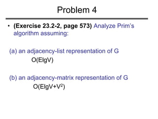
30. (Exercise 23.2-4, page 574): Analyze the
running time of Kruskal’s algorithm when
weights are in the range [1 … V]
Problem 2

31. 1. A ← 
2. for each vertex v  V
3. do MAKE-SET(v)
4. sort E into non-decreasing order by w
5. for each (u, v) taken from the sorted list
6. do if FIND-SET(u)  FIND-SET(v)
7. then A ← A  {(u, v)}
8. UNION(u, v)
9. return A
O(lgV)
O(V)
O(ElgE)
O(E)
- Sorting can be done in O(E) time (e.g., using counting sort)
- However, overall running time will not change, i.e, O(ElgV)
Problem 2 (cont.)

32. Problem 3
• Suppose that some of the weights in a connected
graph G are negative. Will Prim’s algorithm still
work? What about Kruskal’s algorithm? Justify
your answers.
– Yes, both algorithms will work with negative weights.
Review the proof of the generic approach; there is no
assumption in the proof about the weights being
positive.

33. Problem 4
• (Exercise 23.2-2, page 573) Analyze Prim’s
algorithm assuming:
(a) an adjacency-list representation of G
O(ElgV)
(b) an adjacency-matrix representation of G
O(ElgV+V2)

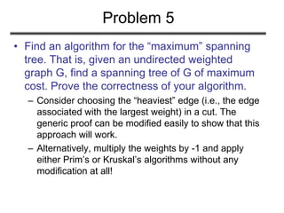
34. PRIM(V, E, w, r)
1. Q ← 
2. for each u  V
3. do key[u] ← ∞
4. π[u] ← NIL
5. INSERT(Q, u)
6. DECREASE-KEY(Q, r, 0) ► key[r] ← 0
7. while Q  
8. do u ← EXTRACT-MIN(Q)
9. for each v  Adj[u]
10. do if v  Q and w(u, v) < key[v]
11. then π[v] ← u
12. DECREASE-KEY(Q, v, w(u, v))
O(V) if Q is implemented
as a min-heap
Executed |V| times
Takes O(lgV)
Min-heap
operations:
O(VlgV)
Executed O(E) times
Constant
Takes O(lgV)
O(ElgV)
Total time: O(VlgV + ElgV) = O(ElgV)
O(lgV)

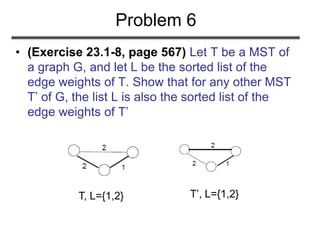
35. PRIM(V, E, w, r)
1. Q ← 
2. for each u  V
3. do key[u] ← ∞
4. π[u] ← NIL
5. INSERT(Q, u)
6. DECREASE-KEY(Q, r, 0) ► key[r] ← 0
7. while Q  
8. do u ← EXTRACT-MIN(Q)
9. for (j=0; j<|V|; j++)
10. if (A[u][j]=1)
11. if v  Q and w(u, v) < key[v]
12. then π[v] ← u
13. DECREASE-KEY(Q, v, w(u, v))
O(V) if Q is implemented
as a min-heap
Executed |V| times
Takes O(lgV)
Min-heap
operations:
O(VlgV)
Executed O(V2) times total
Constant
Takes O(lgV) O(ElgV)
Total time: O(VlgV + ElgV+V2) = O(ElgV+V2)
O(lgV)

36. Problem 5
• Find an algorithm for the “maximum” spanning
tree. That is, given an undirected weighted
graph G, find a spanning tree of G of maximum
cost. Prove the correctness of your algorithm.
– Consider choosing the “heaviest” edge (i.e., the edge
associated with the largest weight) in a cut. The
generic proof can be modified easily to show that this
approach will work.
– Alternatively, multiply the weights by -1 and apply
either Prim’s or Kruskal’s algorithms without any
modification at all!

37. Problem 6
• (Exercise 23.1-8, page 567) Let T be a MST of
a graph G, and let L be the sorted list of the
edge weights of T. Show that for any other MST
T’ of G, the list L is also the sorted list of the
edge weights of T’
T, L={1,2} T’, L={1,2}