Downloaded 271 times


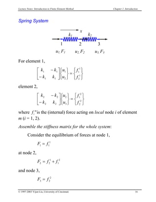
![Lecture Notes: Introduction to Finite Element Method Chapter 1. Introduction
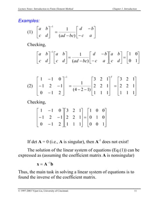
II. Review of Matrix Algebra
Linear System of Algebraic Equations
a x a x a x b
a x a x a x b
a x a x a x b
n n
n n
n n nn n
11 1 12 2 1 1
21 1 22 2 2 2
1 1 2 2
+ +
n
+ =
+ + + =
+ + + =
...
...
.......
...
(1)
where x1, x2, ..., xn are the unknowns.
In matrix form:
Ax (2)b=
where
(3)
[ ]
{ } { }
A
x b
= =
= =
= =
a
a a a
a a a
a a a
x
x
x
x
b
b
b
b
ij
n
n
n n nn
i
n
i
n
11 12 1
21 22 2
1 2
1
2
1
2
...
...
... ... ... ...
...
: :
A is called a n×n (square) matrix, and x and b are (column)
vectors of dimension n.
© 1997-2003 Yijun Liu, University of Cincinnati 7](https://image.slidesharecdn.com/yijunliu-nummeth20040121fem-150216104338-conversion-gate01/85/Yijun-liu-_nummeth_20040121_fem-12-320.jpg)
![Lecture Notes: Introduction to Finite Element Method Chapter 1. Introduction
Row and Column Vectors
v w[ ]= =
v v v
w
w
w
1 2 3
1
2
3
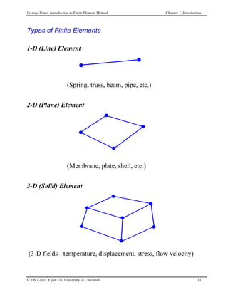
Matrix Addition and Subtraction
For two matrices A and B, both of the same size (m×n), the
addition and subtraction are defined by
ijijij
ijijij
bad
bac
−=−=
+=+=
with
with
BAD
BAC
Scalar Multiplication
[ ]ijaλλ =A
Matrix Multiplication
For two matrices A (of size l×m) and B (of size m×n), the
product of AB is defined by
C kj
m
k
ikij bac ∑=
==
1
withAB
where i = 1, 2, ..., l; j = 1, 2, ..., n.
Note that, in general, AB BA≠ , but (
(associative).
) ( )AB C A BC=
© 1997-2003 Yijun Liu, University of Cincinnati 8](https://image.slidesharecdn.com/yijunliu-nummeth20040121fem-150216104338-conversion-gate01/85/Yijun-liu-_nummeth_20040121_fem-13-320.jpg)
![Lecture Notes: Introduction to Finite Element Method Chapter 1. Introduction
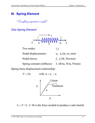
Transpose of a Matrix
If A = [aij], then the transpose of A is
A [ ]T
jia=
Notice that .( )AB B AT T
= T
Symmetric Matrix
A square (n×n) matrix A is called symmetric, if
orA A= T
a aij ji=
Unit (Identity) Matrix
I =
1 0 0
0 1 0
0 0 1
...
...
... ... ... ...
...
Note that AI = A, Ix = x.
Determinant of a Matrix
The determinant of square matrix A is a scalar number
denoted by det A or |A|. For 2×2 and 3×3 matrices, their
determinants are given by
det
a b
c d
ad bc
= −
and
© 1997-2003 Yijun Liu, University of Cincinnati 9](https://image.slidesharecdn.com/yijunliu-nummeth20040121fem-150216104338-conversion-gate01/85/Yijun-liu-_nummeth_20040121_fem-14-320.jpg)
 ( )t a tij=
then the differentiation is defined by
d
dt
t
da t
dt
ij
A( )
( )
=
and the integration by
∫A( ) ( )t dt a t dtij=
∫
© 1997-2003 Yijun Liu, University of Cincinnati 12](https://image.slidesharecdn.com/yijunliu-nummeth20040121fem-150216104338-conversion-gate01/85/Yijun-liu-_nummeth_20040121_fem-17-320.jpg)
![Lecture Notes: Introduction to Finite Element Method Chapter 1. Introduction
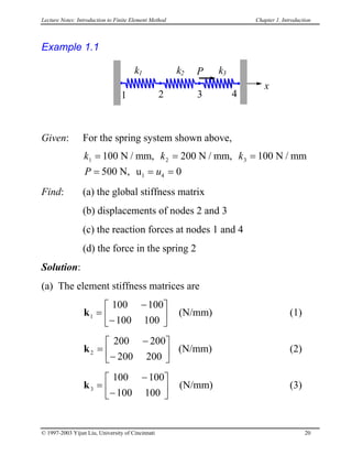
(5)
300 200
200 300
02
3
−
−
=
u
u P
Solving Eq.(5), we obtain
(6)
u
u
P
P
2
3
250
3 500
2
3
=
=
/
/
(mm)
(c) From the 1st
and 4th
equations in (4), we get the reaction forces
F u1 2100 200= − = − (N)
F u4 3100 300= − = − ( )N
(d) The FE equation for spring (element) 2 is
200 200
200 200
−
−
=
u
u
f
f
i
j
i
j
Here i = 2, j = 3 for element 2. Thus we can calculate the spring
force as
[ ]
[ ]
F f f
u
u
j i= = − = −
= −
=
200 200
200 200
2
3
200
2
3
(N)
Check the results!
© 1997-2003 Yijun Liu, University of Cincinnati 22](https://image.slidesharecdn.com/yijunliu-nummeth20040121fem-150216104338-conversion-gate01/85/Yijun-liu-_nummeth_20040121_fem-27-320.jpg)
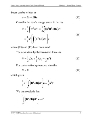
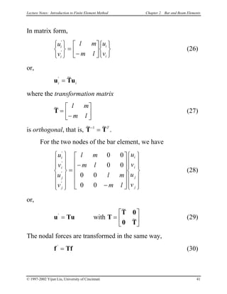
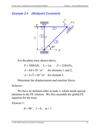
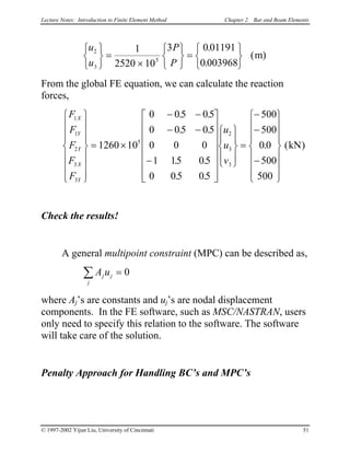
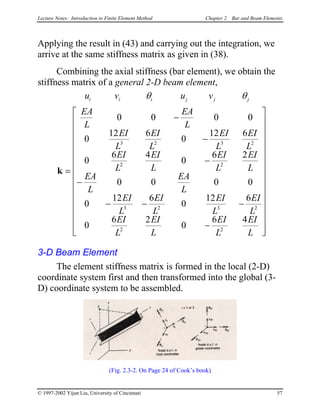
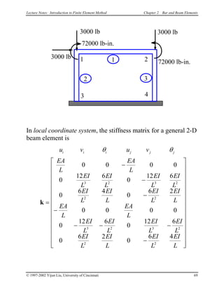
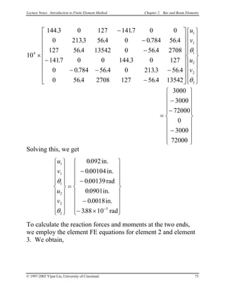
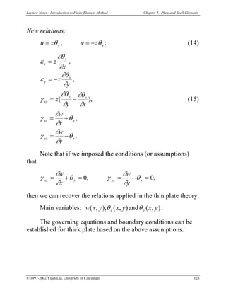
![Lecture Notes: Introduction to Finite Element Method Chapter 2. Bar and Beam Elements
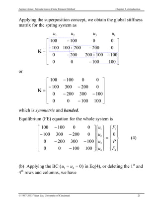
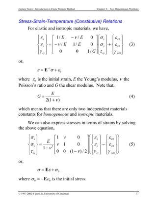
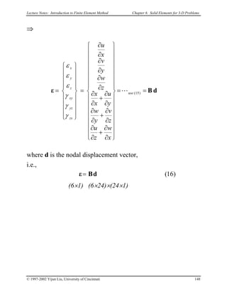
Stiffness Matrix --- A Formal Approach
We derive the same stiffness matrix for the bar using a
formal approach which can be applied to many other more
complicated situations.
Define two linear shape functions as follows
N Ni ( ) , ( )jξ ξ ξ ξ= − =1 (10)
where
ξ =
x
L
, 0 ξ≤ ≤ 1 (11)
From (3) we can write the displacement as
u x u N u N ui i j( ) ( ) ( ) ( )= = j+ξ ξ ξ
or
u N (12)[ ]N
u
ui j
i
j
=
= Nu
Strain is given by (1) and (12) as
ε = =
=
du
dx
d
dx
N u Bu (13)
where B is the element strain-displacement matrix, which is
[ ] [ ]B = =
d
dx
N N
d
d
N N
d
dx
i j i j( ) ( ) ( ) ( )ξ ξ
ξ
ξ ξ •
ξ
i.e., (14)[B = −1 1/ /L ]L
© 1997-2002 Yijun Liu, University of Cincinnati 29](https://image.slidesharecdn.com/yijunliu-nummeth20040121fem-150216104338-conversion-gate01/85/Yijun-liu-_nummeth_20040121_fem-34-320.jpg)
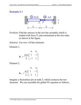
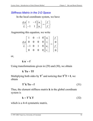
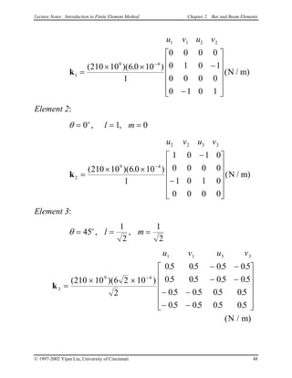
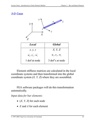
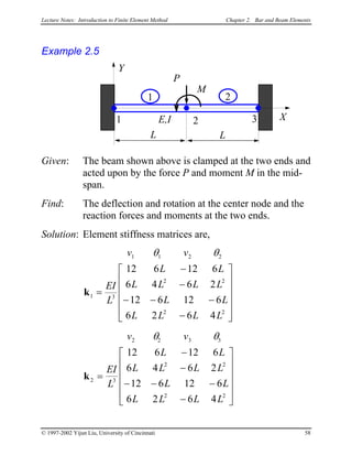
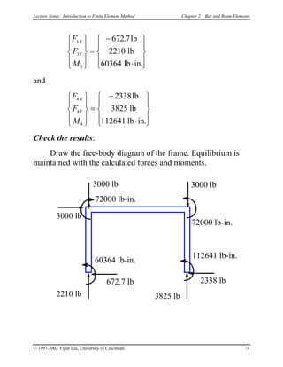
![Lecture Notes: Introduction to Finite Element Method Chapter 2. Bar and Beam Elements
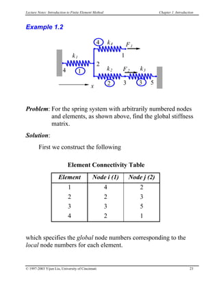
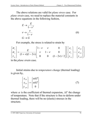
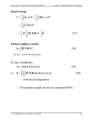
or
ku f= (19)
where
(20)( )k B BT
=
∫ E dV
V
is the element stiffness matrix.
Expression (20) is a general result which can be used for
the construction of other types of elements. This expression can
also be derived using other more rigorous approaches, such as
the Principle of Minimum Potential Energy, or the Galerkin’s
Method.
Now, we evaluate (20) for the bar element by using (14)
[ ]k =
−
− =
−
−
∫
1
1
1 1
1 1
1 1
0
/
/
/ /
L
L
E L L Adx
EA
L
L
which is the same as we derived using the direct method.
Note that from (16) and (20), the strain energy in the
element can be written as
U (21)=
1
2
u kuT
© 1997-2002 Yijun Liu, University of Cincinnati 31](https://image.slidesharecdn.com/yijunliu-nummeth20040121fem-150216104338-conversion-gate01/85/Yijun-liu-_nummeth_20040121_fem-36-320.jpg)
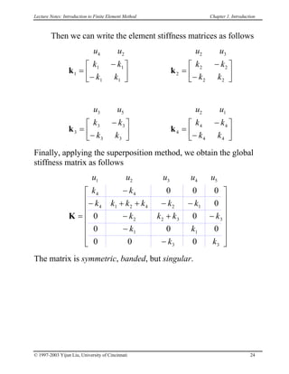
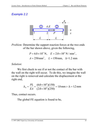
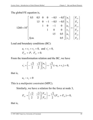
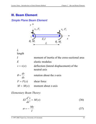
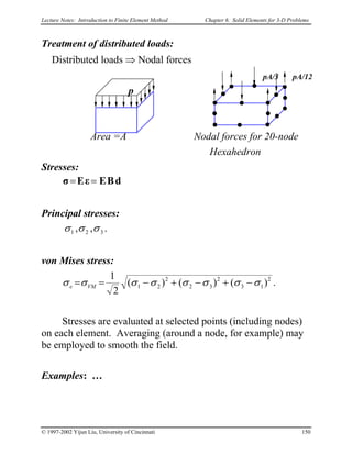
![Lecture Notes: Introduction to Finite Element Method Chapter 2. Bar and Beam Elements
EA
L
u
u
u
F
F
F
2 2 0
2 3 1
0 1 1
1
2
3
1
2
3
−
− −
−
=
Load and boundary conditions (BC) are,
u u F P1 3 20= = =,
FE equation becomes,
EA
L
u
F
P
F
2 2 0
2 3 1
0 1 1
0
0
2
1
3
−
− −
−
=
Deleting the 1st
row and column, and the 3rd
row and column, we
obtain,
[ ]{ } { }
EA
L
u P3 2 =
Thus,
u
PL
EA
2
3
=
and
u
u
u
PL
EA
1
2
3
3
0
1
0
=
Stress in element 1 is
© 1997-2002 Yijun Liu, University of Cincinnati 33](https://image.slidesharecdn.com/yijunliu-nummeth20040121fem-150216104338-conversion-gate01/85/Yijun-liu-_nummeth_20040121_fem-38-320.jpg)
![Lecture Notes: Introduction to Finite Element Method Chapter 2. Bar and Beam Elements
[ ]σ ε1 1 1 1
1
2
2 1
1 1
3
0
3
= = = −
=
−
= −
=
E E E L L
u
u
E
u u
L
E
L
PL
EA
P
A
B u / /
Similarly, stress in element 2 is
[ ]σ ε2 2 2 2
2
3
3 2
1 1
0
3 3
= = = −
=
−
= −
= −
E E E L L
u
u
E
u u
L
E
L
PL
EA
P
A
B u / /
which indicates that bar 2 is in compression.
Check the results!
Notes:
• In this case, the calculated stresses in elements 1 and 2
are exact within the linear theory for 1-D bar structures.
It will not help if we further divide element 1 or 2 into
smaller finite elements.
• For tapered bars, averaged values of the cross-sectional
areas should be used for the elements.
• We need to find the displacements first in order to find
the stresses, since we are using the displacement based
FEM.
© 1997-2002 Yijun Liu, University of Cincinnati 34](https://image.slidesharecdn.com/yijunliu-nummeth20040121fem-150216104338-conversion-gate01/85/Yijun-liu-_nummeth_20040121_fem-39-320.jpg)
![Lecture Notes: Introduction to Finite Element Method Chapter 2. Bar and Beam Elements
EA
L
u
u
u
F
F
F
1 1 0
1 2 1
0 1 1
1
2
3
1
2
3
−
− −
−
=
The load and boundary conditions are,
F P
u u
2
4
1 3
6 0 10
0 1
= = ×
= = =
.
, .
N
mm∆ 2
FE equation becomes,
EA
L
u
F
P
F
1 1 0
1 2 1
0 1 1
0
2
1
3
−
− −
−
=
∆
The 2nd
equation gives,
[ ] { }
EA
L
u
P2 1 2
−
=
∆
that is,
[ ]{ }
EA
L
u P
EA
L
2 2 = +
∆
Solving this, we obtain
u
PL
EA
2
1
2
15= +
=∆ . mm
and
© 1997-2002 Yijun Liu, University of Cincinnati 36](https://image.slidesharecdn.com/yijunliu-nummeth20040121fem-150216104338-conversion-gate01/85/Yijun-liu-_nummeth_20040121_fem-41-320.jpg)
![Lecture Notes: Introduction to Finite Element Method Chapter 2. Bar and Beam Elements
u
u
u
1
2
3
0
15
12
=
.
.
( )mm
To calculate the support reaction forces, we apply the 1st
and 3rd
equations in the global FE equation.
The 1st
equation gives,
[ ] ( )
EA
L
u
u
u
EA
L
u1
1
2
3
2
4
1 1 0 50 10= −
= − = − ×. NF
and the 3rd
equation gives,
[ ] ( )F
EA
L
u
u
u
EA
L
u u3
1
2
3
2 3
4
0 1 1
10 10
= −
= − +
= − ×. N
Check the results.!
© 1997-2002 Yijun Liu, University of Cincinnati 37](https://image.slidesharecdn.com/yijunliu-nummeth20040121fem-150216104338-conversion-gate01/85/Yijun-liu-_nummeth_20040121_fem-42-320.jpg)
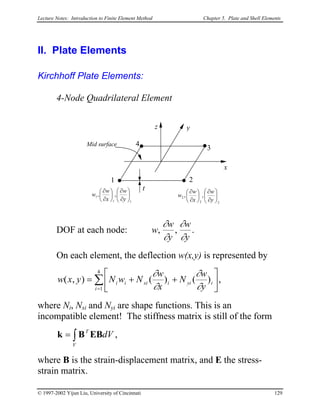
![Lecture Notes: Introduction to Finite Element Method Chapter 2. Bar and Beam Elements
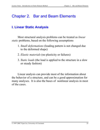
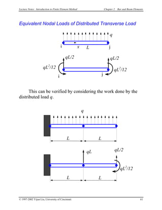
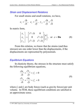
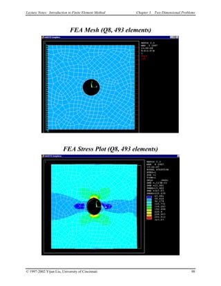
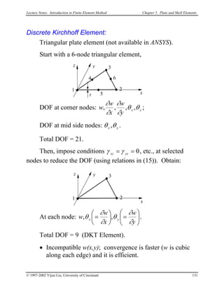
Distributed Load
x
i j
q
qL/2
i j
qL/2
Uniformly distributed axial load q (N/mm, N/m, lb/in) can
be converted to two equivalent nodal forces of magnitude qL/2.
We verify this by considering the work done by the load q,
[ ]
[ ]
[ ]
W uqdx u q Ld
qL
u d
qL
N N
u
u
d
qL
d
u
u
qL qL u
u
u u
qL
qL
q
L
i j
i
j
i
j
i
j
i j
= = =
=
= −
=
=
∫ ∫ ∫
∫
∫
1
2
1
2 2
2
2
1
1
2 2 2
1
2
2
2
0 0
1
0
1
0
1
0
1
( ) ( ) ( )
( ) ( )
/
/
ξ ξ ξ
ξ ξ ξ
ξ ξ ξ
ξ
© 1997-2002 Yijun Liu, University of Cincinnati 38](https://image.slidesharecdn.com/yijunliu-nummeth20040121fem-150216104338-conversion-gate01/85/Yijun-liu-_nummeth_20040121_fem-43-320.jpg)
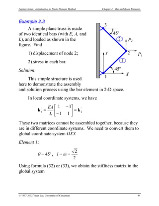
![Lecture Notes: Introduction to Finite Element Method Chapter 2. Bar and Beam Elements
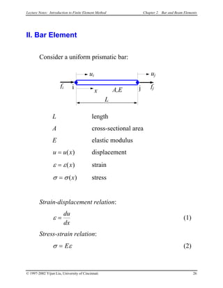
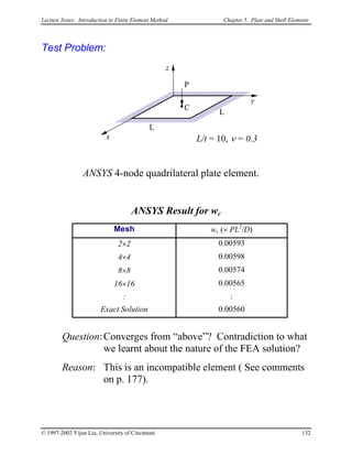
Bar Elements in 2-D and 3-D Space
2-D Case
x
i
j
ui
’
y
X
Y
θ
ui
vi
Local Global
x, y X, Y
u vi i
' '
, u vi i,
1 dof at a node 2 dof’s at a node
Note: Lateral displacement vi
’
does not contribute to the stretch
of the bar, within the linear theory.
Transformation
[ ]
[ ]
u u v l m
u
v
v u v m l
u
v
i i i
i
i
i i i
i
i
'
'
cos sin
sin cos
= + =
= − + = −
θ θ
θ θ
where l m= =cos , sinθ θ .
© 1997-2002 Yijun Liu, University of Cincinnati 40](https://image.slidesharecdn.com/yijunliu-nummeth20040121fem-150216104338-conversion-gate01/85/Yijun-liu-_nummeth_20040121_fem-45-320.jpg)
![Lecture Notes: Introduction to Finite Element Method Chapter 2. Bar and Beam Elements
Explicit form,
u v u v
EA
L
l lm l l
lm m lm m
l lm l lm
lm m lm m
i i j
k =
− −
− −
− −
− −
2 2
2
2 2
2 2
m
j
2
(33)
Calculation of the directional cosines l and m:
l
X X
L
m
Y Y
L
j i j
= = i−
= =
−
cos , sinθ θ (34)
The structure stiffness matrix is assembled by using the element
stiffness matrices in the usual way as in the 1-D case.
Element Stress
σ ε= =
= −
E E
u
u
E
L L
l m
l m
u
v
u
v
i
j
i
i
j
j
B
'
'
1 1 0 0
0 0
That is,
[σ = − −
E
L
l m l m
u
v
u
v
i
i
j
j
] (35)
© 1997-2002 Yijun Liu, University of Cincinnati 43](https://image.slidesharecdn.com/yijunliu-nummeth20040121fem-150216104338-conversion-gate01/85/Yijun-liu-_nummeth_20040121_fem-48-320.jpg)
![Lecture Notes: Introduction to Finite Element Method Chapter 2. Bar and Beam Elements
Load and boundary conditions (BC):
u v u v F P F PX Y1 1 3 3 2 1 20= = = 2= = =, ,
Condensed FE equation,
EA
L
u
v
P
P2
2 0
0 2
2
2
1
2
=
Solving this, we obtain the displacement of node 2,
u
v
L
EA
P
P
2
2
1
2
=
Using formula (35), we calculate the stresses in the two bars,
[ ] ( )σ1
1
2
1 2
2
2
1 1 1 1
0
0 2
2
= − −
= +
E
L
L
EA P
P
A
P P
[ ] ( )σ2
1
2
1 2
2
2
1 1 1 1
0
0
2
2
= − −
= −
E
L
L
EA
P
P
A
P P
Check the results:
Look for the equilibrium conditions, symmetry,
antisymmetry, etc.
© 1997-2002 Yijun Liu, University of Cincinnati 46](https://image.slidesharecdn.com/yijunliu-nummeth20040121fem-150216104338-conversion-gate01/85/Yijun-liu-_nummeth_20040121_fem-51-320.jpg)
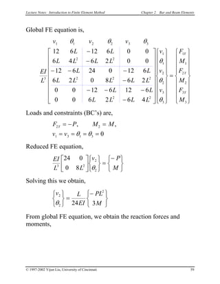
![Lecture Notes: Introduction to Finite Element Method Chapter 2. Bar and Beam Elements
Formal Approach
Apply the formula,
(39)k B B=
∫
T
L
EI dx
0
To derive this, we introduce the shape functions,
(40)
N x x L x L
N x x x L x L
N x x L x L
N x x L x L
1
2 2 3
2
2 3
3
2 2 3 3
4
2 3 2
1 3 2
2
3 2
( ) / /
( ) / /
( ) / /
( ) / /
= − +
= − +
= −
= − +
3
2
Then, we can represent the deflection as,
(41)
[ ]
v x
N x N x N x N x
v
v
i
i
j
j
( )
( ) ( ) ( ) ( )
=
=
Nu
1 2 3 4
θ
θ
which is a cubic function. Notice that,
N N
N N L N
1 3
2 3 4
1+ =
+ + = x
which implies that the rigid body motion is represented by the
assumed deformed shape of the beam.
© 1997-2002 Yijun Liu, University of Cincinnati 55](https://image.slidesharecdn.com/yijunliu-nummeth20040121fem-150216104338-conversion-gate01/85/Yijun-liu-_nummeth_20040121_fem-60-320.jpg)
![Lecture Notes: Introduction to Finite Element Method Chapter 2. Bar and Beam Elements
Curvature of the beam is,
d v
dx
d
dx
2
2
2
2
= =Nu Bu (42)
where the strain-displacement matrix B is given by,
[ ]B N= =
= − + − + − − +
d
dx
N x N x N x N x
L
x
L L
x
L L
x
L L
x
L
2
2 1 2 3 4
2 3 2 2 3 2
6 12 4 6 6 12 2 6
" " " "
( ) ( ) ( ) ( )
(43)
Strain energy stored in the beam element is
( ) ( )
U dV
My
I E
My
I
dAdx
M
EI
Mdx
d v
dx
EI
d v
dx
dx
EI dx
EI dx
T
V A
L T
T
L TL
T
L
T T
L
= = −
−
= =
=
=
∫ ∫∫
∫ ∫
∫
∫
1
2
1
2
1
1
2
1 1
2
1
2
1
2
0
0
2
2
2
2
0
0
0
σ ε
Bu Bu
u B B u
We conclude that the stiffness matrix for the simple beam
element is
k B B=
∫
T
L
EI dx
0
© 1997-2002 Yijun Liu, University of Cincinnati 56](https://image.slidesharecdn.com/yijunliu-nummeth20040121fem-150216104338-conversion-gate01/85/Yijun-liu-_nummeth_20040121_fem-61-320.jpg)
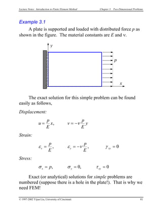
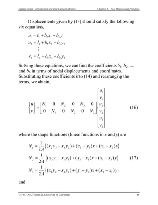
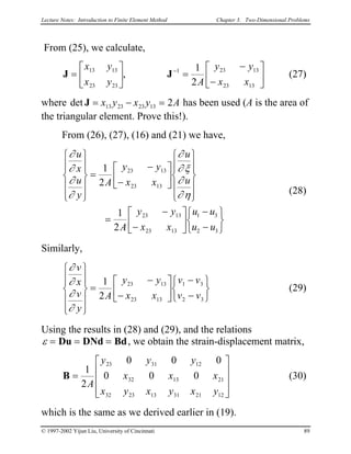
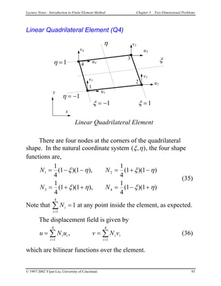
![Lecture Notes: Introduction to Finite Element Method Chapter 3. Two-Dimensional Problems
u s s L u s L un nA( ) ( / ) ( / )= − nB+1
The traction q(s), which is also linear, is given in a similar way,
q s s L q s L qA B( ) ( / ) ( / )= − +1
Thus, we have,
[ ] [ ]
[ ]
[ ]
W t u u
s L
s L
s L s L
q
q
ds
u u t
s L s L s L
s L s L s L
ds
q
q
u u
tL q
q
q nA nB
A
B
L
nA nB
L
A
B
nA nB
A
B
=
−
−
=
− −
−
=
∫
∫
1
1
1 1
1
6
2 1
1 2
0
2
2
0
/
/
/ /
( / ) ( / )( / )
( / )( / ) ( / )
and the equivalent nodal force vector is,
f
f
tL q
q
A
B
A
B
=
6
2 1
1 2
Note, for constant q, we have,
f
f
qtLA
B
=
2
1
1
For quadratic elements (either triangular or quadrilateral),
the traction is converted to forces at three nodes along the edge,
instead of two nodes.
Traction tangent to the boundary, as well as body forces,
are converted to nodal forces in a similar way.
© 1997-2002 Yijun Liu, University of Cincinnati 100](https://image.slidesharecdn.com/yijunliu-nummeth20040121fem-150216104338-conversion-gate01/85/Yijun-liu-_nummeth_20040121_fem-105-320.jpg)
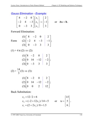
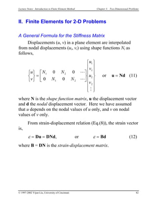
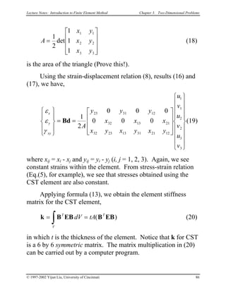
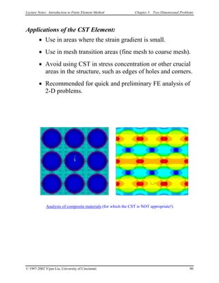
![Lecture Notes: Introduction to Finite Element Method Chapter 4. FE Modeling and Solution Techniques
Iterative Method - Example:
The Gauss-Seidel Method
bAx = (A is symmetric)
or ....,,2,1,
1
Nibxa
N
j
ijij ==∑
=
Start with an estimate and then iterate using the following:)( 0
x
....,,2,1for
,
1 1
1 1
)()1()1(
Ni
xaxab
a
x
i
j
N
ij
k
jij
k
jiji
ii
k
i
=
−−= ∑ ∑
−
= +=
++
In vector form,
[ ],)()1(1)1( kT
L
k
LD
k
xAxAbAx −−= +−+
where
〉〈= iiD aA is the diagonal matrix of A,
LA is the lower triangular matrix of A,
such that A .
T
LLD AAA ++=
Iterations continue until solution x converges, i.e.
,)(
)()1(
ε≤
−+
k
kk
x
xx
where ε is the tolerance for convergence control.
© 1997-2002 Yijun Liu, University of Cincinnati 111](https://image.slidesharecdn.com/yijunliu-nummeth20040121fem-150216104338-conversion-gate01/85/Yijun-liu-_nummeth_20040121_fem-116-320.jpg)
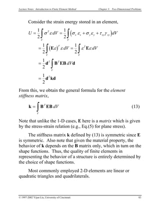
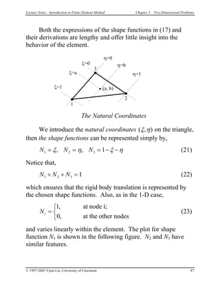
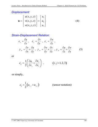
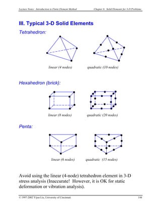
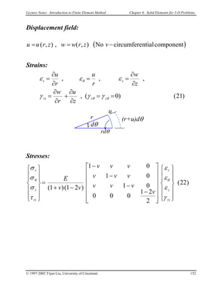
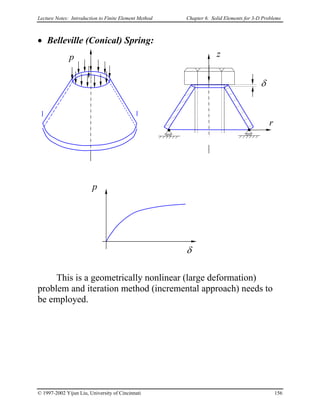
![Lecture Notes: Introduction to Finite Element Method Chapter 6. Solid Elements for 3-D Problems
{ } [ ] )1(, ij
zx
yz
xy
z
y
x
or σ
τ
τ
τ
σ
σ
σ
σ
==σ
Strains:
{ } [ ] )2(, ij
zx
yz
xy
z
y
x
or ε
γ
γ
γ
ε
ε
ε
ε
==ε
Stress-strain relation:
−
−
−
−
−
−
−+
=
zx
yz
xy
z
y
x
zx
yz
xy
z
y
x
v
v
v
vvv
vvv
vvv
vv
E
γ
γ
γ
ε
ε
ε
τ
τ
τ
σ
σ
σ
2
21
00000
0
2
21
0000
00
2
21
000
0001
0001
0001
)21)(1(
or )3(Eεσ =
© 1997-2002 Yijun Liu, University of Cincinnati 139](https://image.slidesharecdn.com/yijunliu-nummeth20040121fem-150216104338-conversion-gate01/85/Yijun-liu-_nummeth_20040121_fem-144-320.jpg)
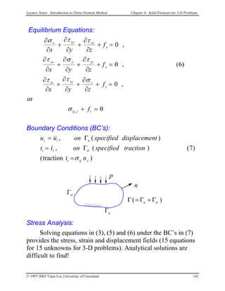
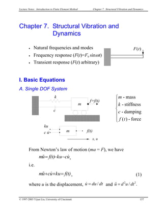
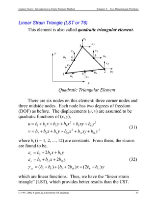
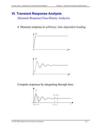
![Lecture Notes: Introduction to Finite Element Method Chapter 7. Structural Vibration and Dynamics
Free Vibration: f(t) = 0 and no damping (c = 0)
Eq. (1) becomes
0=+ ukum&& . (2)
(meaning: inertia force + stiffness force = 0)
Assume:
t)(Uu(t) ωsin= ,
where ω is the frequency of oscillation, U the amplitude.
Eq. (2) yields
0sinsin2
=+− t)ω(Ukt)ω(mωU
i.e.,
[ ] 02
=+− Ukmω .
For nontrivial solutions for U, we must have
[ ] 02
=+− kmω ,
which yields
m
k
=ω . (3)
This is the circular natural frequency of the single DOF
system (rad/s). The cyclic frequency (1/s = Hz) is
π
ω
2
=f , (4)
© 1997-2003 Yijun Liu, University of Cincinnati 158](https://image.slidesharecdn.com/yijunliu-nummeth20040121fem-150216104338-conversion-gate01/85/Yijun-liu-_nummeth_20040121_fem-163-320.jpg)
![Lecture Notes: Introduction to Finite Element Method Chapter 7. Structural Vibration and Dynamics
© 1997-2003 Yijun Liu, University of Cincinnati 161
In general, we have the consistent mass matrix given by
(9)dV
V
T
∫= NNm ρ
where N is the same shape function matrix as used for the
displacement field.
This is obtained by considering the kinetic energy:
( )
( ) ( )
uNNu
uNuN
umu
m
&
43421
&
&&
&&&
&&
∫
∫
∫∫
=
=
==
=Κ
V
TT
V
T
V
T
V
T
dV
dV
dVuudVu
mv
ρ
ρ
ρρ
2
1
2
1
2
1
2
1
)
2
1
(cf.
2
1
2
2
Bar Element (linear shape function):
(10)
[ ]
3/16/1
6/13/1
1
1
2
1
u
u
AL
ALd
V
&&
&&
=
−
−
= ∫
ρ
ξξξ
ξ
ξ
ρm
Element mass matrices:
⇒ local coordinates ⇒ to global coordinates
⇒ assembly of the global structure mass matrix M.](https://image.slidesharecdn.com/yijunliu-nummeth20040121fem-150216104338-conversion-gate01/85/Yijun-liu-_nummeth_20040121_fem-166-320.jpg)
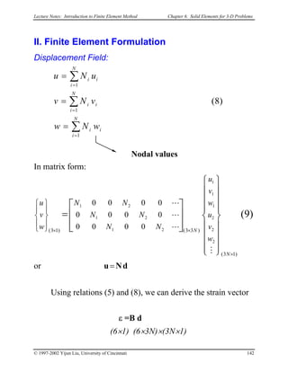
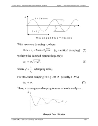
![Lecture Notes: Introduction to Finite Element Method Chapter 7. Structural Vibration and Dynamics
II. Free Vibration
Study of the dynamic characteristics of a structure:
• natural frequencies
• normal modes (shapes)
Let f(t) = 0 and C = 0 (ignore damping) in the dynamic
equation (8) and obtain
0KuuM =+&& (12)
Assume that displacements vary harmonically with time, that
is,
),sin()(
),cos()(
),sin()(
2
tt
tt
tt
ωω
ωω
ω
uu
uu
uu
−=
=
=
&&
&
where u is the vector of nodal displacement amplitudes.
Eq. (12) yields,
[ ] 0uMK =− 2
ω (13)
This is a generalized eigenvalue problem (EVP).
Solutions?
© 1997-2003 Yijun Liu, University of Cincinnati 163](https://image.slidesharecdn.com/yijunliu-nummeth20040121fem-150216104338-conversion-gate01/85/Yijun-liu-_nummeth_20040121_fem-168-320.jpg)
![Lecture Notes: Introduction to Finite Element Method Chapter 7. Structural Vibration and Dynamics
Trivial solution: 0u = for any values of ω (not interesting).
Nontrivial solutions: 0u ≠ only if
02
=− MK ω (14)
This is an n-th order polynomial of ω2
, from which we can
find n solutions (roots) or eigenvalues ωi.
ωi (i = 1, 2, …, n) are the natural frequencies (or
characteristic frequencies) of the structure.
ω1 (the smallest one) is called the fundamental frequency.
For each ωi , Eq. (13) gives one solution (or eigen) vector
[ ] 0uMK =− ii
2
ω .
iu (i=1,2,…,n) are the normal modes (or natural modes,
mode shapes, etc.).
Properties of Normal Modes
0=j
T
i uKu ,
0=j
T
i uMu , for i ≠ j, (15)
if ji ωω ≠ . That is, modes are orthogonal (or independent) to
each other with respect to K and M matrices.
© 1997-2003 Yijun Liu, University of Cincinnati 164](https://image.slidesharecdn.com/yijunliu-nummeth20040121fem-150216104338-conversion-gate01/85/Yijun-liu-_nummeth_20040121_fem-169-320.jpg)
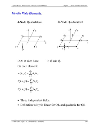
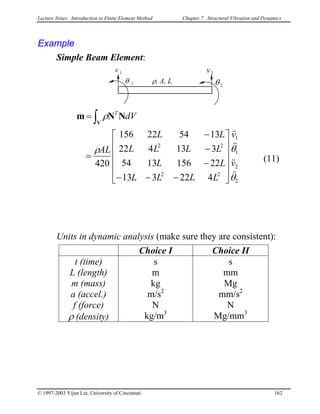
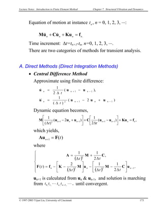
![Lecture Notes: Introduction to Finite Element Method Chapter 7. Structural Vibration and Dynamics
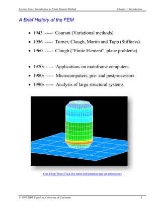
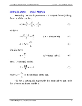
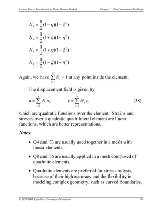
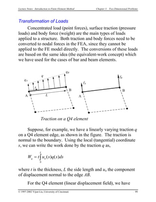
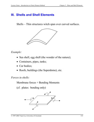
Example:
L
x1 2
v2
ρ, A, EI
y
θ2
[ ]
.
422
22156
420
,
46
612
,
0
0
223
2
22
−
−
=
−
−
=
=
−
LL
LAL
LL
L
L
EI
v
ρ
θ
ω
MK
MK
EVP:
in which λ = .EIAL 420/42
ρω
,0
44226
22615612
22
=
−+−
+−−
λλ
λλ
LLLL
LL
Solving the EVP, we obtain,
.62.7
1v
,81.34
,38.1
1v
,533.3
22
2
2
1
42
12
2
2
1
41
=
=
=
=
LAL
EI
LAL
EI
θρ
ω
θρ
ω
#1
#2#3
Exact solutions:
.03.22,516.3
2
1
42
2
1
41
=
=
AL
EI
AL
EI
ρ
ω
ρ
ω
We can see that mode 1 is calculated much more accurately
than mode 2, with one beam element.
© 1997-2003 Yijun Liu, University of Cincinnati 166](https://image.slidesharecdn.com/yijunliu-nummeth20040121fem-150216104338-conversion-gate01/85/Yijun-liu-_nummeth_20040121_fem-171-320.jpg)
![Lecture Notes: Introduction to Finite Element Method Chapter 7. Structural Vibration and Dynamics
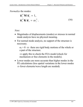
IV. Modal Equations
Use the normal modes (modal matrix) to transform the
coupled system of dynamic equations to uncoupled system of
equations.
We have
[ ] n1,2,...,,
2
==− iii 0uMK ω (18)
where the normal mode iu satisfies:
=
=
,0
,0
j
T
i
j
T
i
uMu
uKu
for i ≠ j,
and
=
=
,
,1
2
ii
T
i
i
T
i
ωuKu
uMu
for i = 1, 2, …, n.
Form the modal matrix:
[ ]nnn uuuΦ 21)( L=× (19)
We can verify that
.
,matrix)Spectral(
00
0
0
00
2
n
2
2
2
1
IMΦΦ
ΩKΦΦ
=
==
T
T
ω
ω
ω
L
OM
M
L
(20)
Transformation for the displacement vector,
zuuuu Φ=+++= nnzzz L2211 , (21)
© 1997-2003 Yijun Liu, University of Cincinnati 168](https://image.slidesharecdn.com/yijunliu-nummeth20040121fem-150216104338-conversion-gate01/85/Yijun-liu-_nummeth_20040121_fem-173-320.jpg)
![Lecture Notes: Introduction to Finite Element Method Chapter 7. Structural Vibration and Dynamics
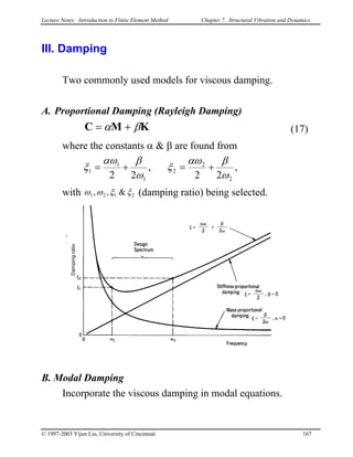
V. Frequency Response Analysis
(Harmonic Response Analysis)
321&&&
loadingHarmonic
sin tωFKuuCuM =++
(25)
Modal method: Apply the modal equations,
i=1,2,…,m. (26)
These are 1-D equations. Solutions are
,sin2 2
tpzzz iiiiiii ωωωξ =++ &&&
),sin(
)2()1(
)(
222
2
i
iii
ii
i t
p
tz θω
ηξη
ω
−
+−
= (27)
i
where
z
ω/ωi
==
=
−
=
ratiodamping,
2
,
anglephase,
1
2
arctan
i
2
i
i
c
i
i
i
i
ii
i
m
c
c
c
ω
ξ
ωωη
η
ηξ
θ
Recover u from (21).
Direct Method: Solve Eq. (25) directly, that is, calculate the
inverse. With
ti
e ω
uu = (complex notation), Eq. (25)
becomes
[ ] .2
FuMCK =−+ ωωi
This equation is expensive to solve and matrix is ill-
conditioned if ω is close to any ωi.
© 1997-2003 Yijun Liu, University of Cincinnati 171](https://image.slidesharecdn.com/yijunliu-nummeth20040121fem-150216104338-conversion-gate01/85/Yijun-liu-_nummeth_20040121_fem-176-320.jpg)
![Lecture Notes: Introduction to Finite Element Method Chapter 7. Structural Vibration and Dynamics
This method is unstable if ∆t is too large.
• Newmark Method:
Use approximations:
[ ]
[ ],)1(
)(,2)21(
2
)(
11
11
2
1
++
+++
+−∆+≈
=→+−
∆
+∆+≈
nnnn
nnnnnn
t
t
t
uuuu
uuuuuu
&&&&&&
L&&&&&&&
γγ
ββ
where β & γ are chosen constants. These lead to
)(1 tn FAu =+
where
).,,,,,,,,()(
,
)(
1
1
2
nnnn tft
tt
uuuMCfF
MCKA
&&&∆=
∆
+
∆
+=
+ βγ
ββ
γ
This method is unconditionally stable if
4
1
,
2
1
.,.e
.
2
1
2
==
≥≥
βγ
γβ
g
which gives the constant average acceleration method.
Direct methods can be expensive! (the need to compute
A-1
, often repeatedly for each time step).
© 1997-2003 Yijun Liu, University of Cincinnati 174](https://image.slidesharecdn.com/yijunliu-nummeth20040121fem-150216104338-conversion-gate01/85/Yijun-liu-_nummeth_20040121_fem-179-320.jpg)
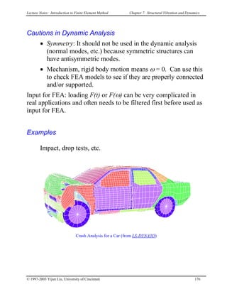

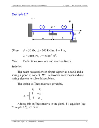
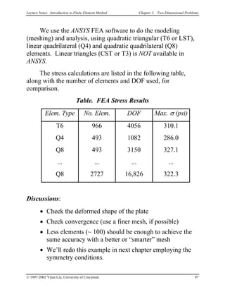
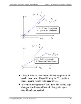
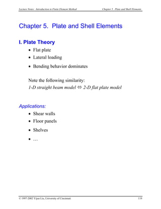
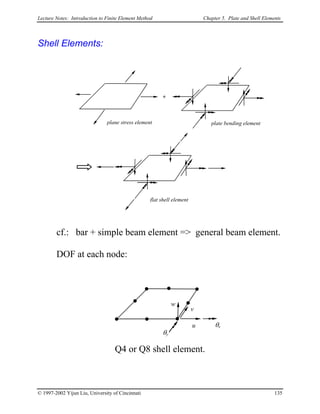
The document provides an introduction to the finite element method (FEM) through lecture notes. It discusses the basic concepts of dividing a complex problem into smaller, simpler pieces called finite elements. The history and applications of FEM in engineering are described, including using FEM for structural analysis which involves dividing a structure into finite elements connected at nodes. The table of contents outlines the topics that will be covered in the subsequent chapters, such as bar, beam, plate, shell and solid elements, as well as structural dynamics, vibration and thermal analysis using FEM.


![Assignment [4] machining with solutions](https://cdn.slidesharecdn.com/ss_thumbnails/assignment4machining-withsolutions-121213110841-phpapp02-thumbnail.jpg?width=640&height=640&fit=bounds)