Downloaded 3,970 times


![Forme d’auge Angle Section de char- Comparai-
d’auge gement A(m2) son
plat 0,0483 44%
20° 0,1007 91%
30° 0,1145 104%
20° 0,0935 85%
30° 0,1100 100%
45° 0,1247 113%
20° 0,0989 90%
30° 0,1161 106%
45° 0,1284 117%
30°/60° 0,1329 121%
Auge profonde
Guirlande
11.5
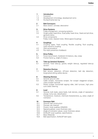
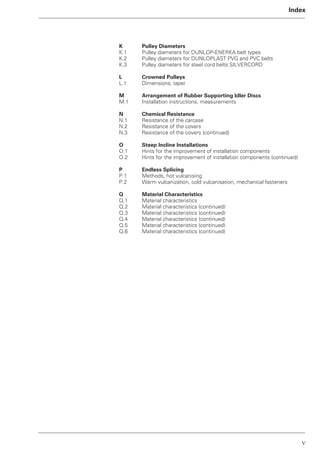
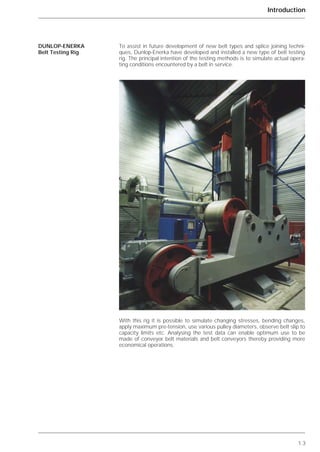
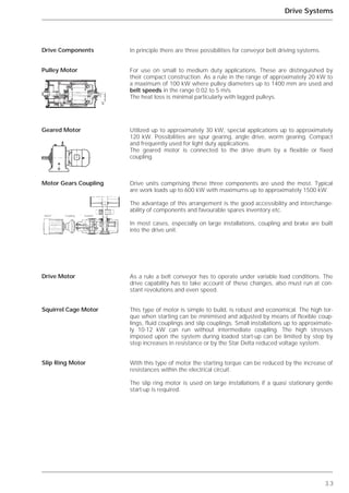
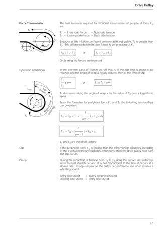
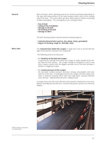
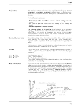
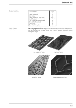
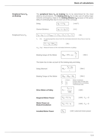
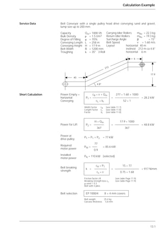
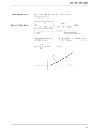
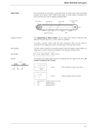
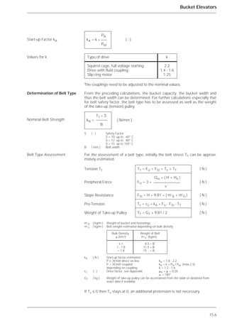
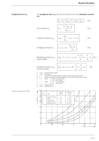
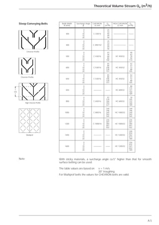
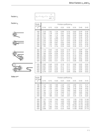
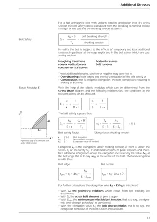
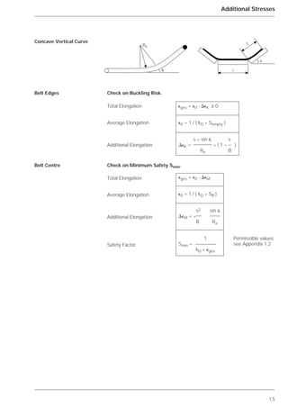
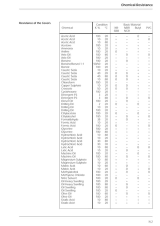
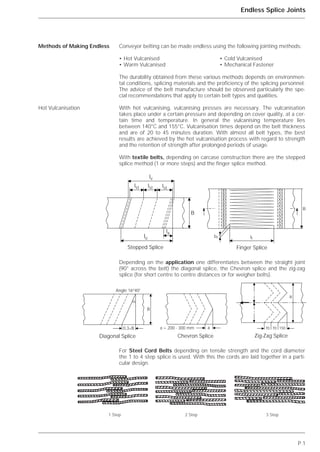
Design
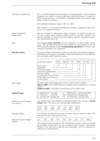
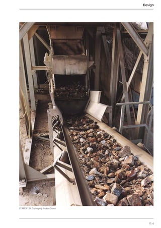
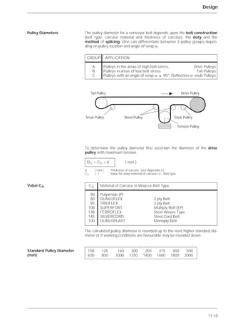
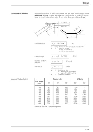
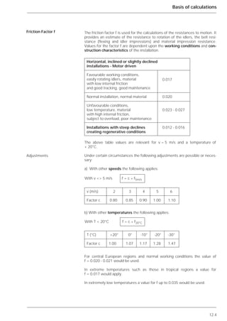
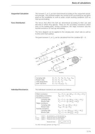
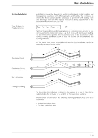
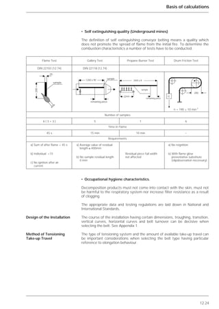
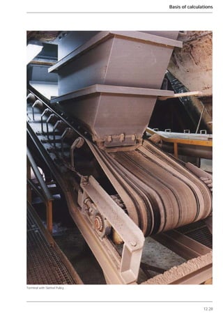
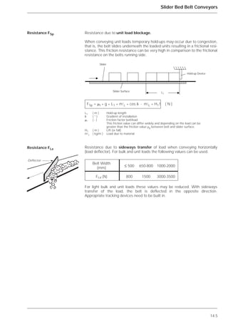
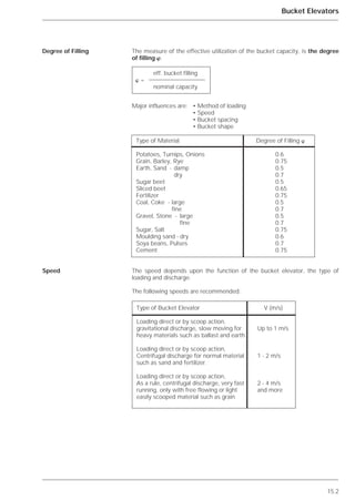
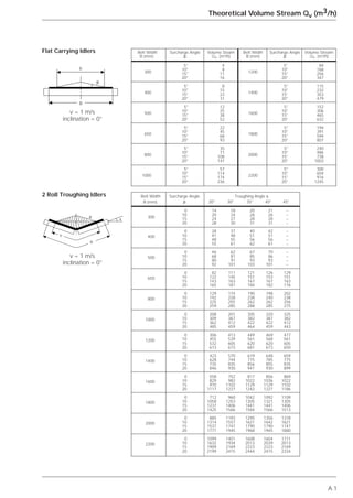
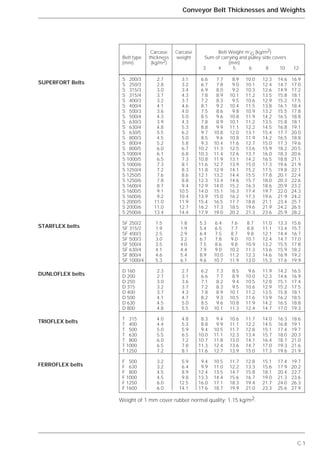
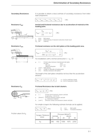
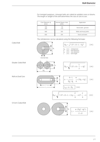
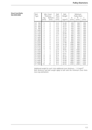
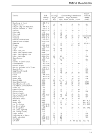
To determine the cross-sectional area of the load stream A, one may use as a
basis the geometric relationship which can be constructed from the troughing
angle , the usable belt width b and the angle of surcharge ß.
For 1, 2 and 3 roll carrying idler sets, the part cross-sectional area can be cal-
culated as follows:
Cross Sectional Area of
Load Stream
Cross-Sectional Area of
Load Stream
Part Cross-Sectional
Area
Cross Sectional Area
Comparison for Various
Forms of Troughing.
Note:
The values for the cross sec-
tional area and the compari-
son are for a belt width B =
1000 mm and for an angle of
surcharge  = 15°.
B
b
l

l1
A2
A1
᭤
᭣ ᭣
᭣
᭣ ᭤
᭤
᭣
᭤
᭣
᭤᭣
A = A1 + A2 ( m2 )
A1 = 0.25 * tan  * [ l + ( b - l ) * cos ]2 ( m2 )
A2 = l1 * sin * [ l + l1 * cos ] ( m2 )
l ( m ) Length of middle carrying roll
l1 ( m ) Loading width of outer rolls
l1 = 0.5 ( b - l ) for 3 roll idler sets
l1 = 0.5 ( b - 3 * l )for 5 roll Garland sets
b ( m ) Usable belt width (loadstream width)
b = 0.9 * B - 50 mm for belts B ≤ 2000 mm
b = B - 250 mm for belts B > 2200 mm
( ° ) Troughing Angle
 ( ° ) Surcharge Angle
Troughing Form Troughing
Angle
Load Cross Sec-
tion Area A(M2
)
Compari-
son
Flat
Deep Trough
Garland
0.0483
0.1329
0.1007
0.1145
0.0935
0.1100
0.1247
0.0989
0.1161
0.1284](https://image.slidesharecdn.com/beltconveyordesign-dunlop-140630061205-phpapp02/85/Belt-conveyor-design-dunlop-39-320.jpg)

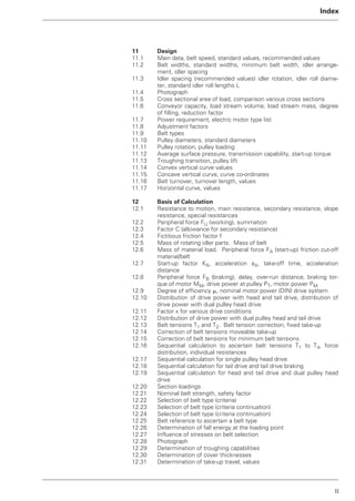
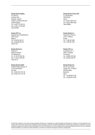
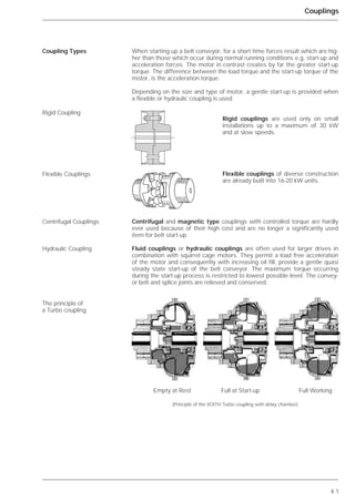
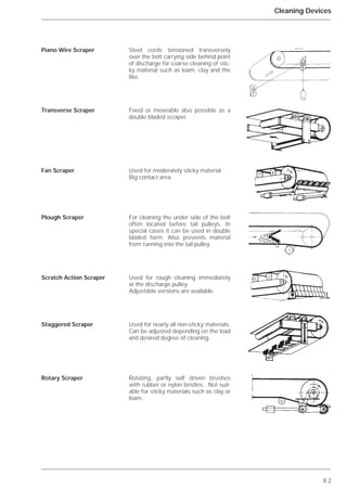
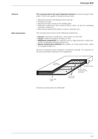
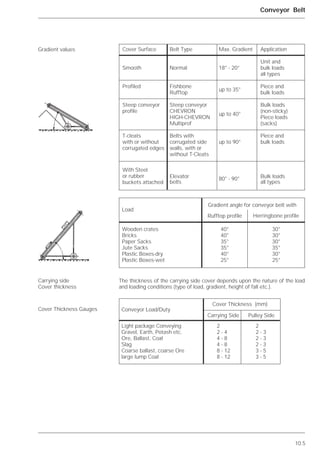
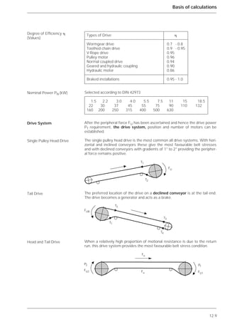
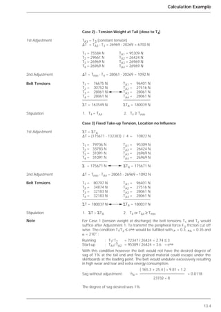
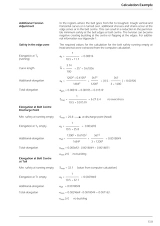
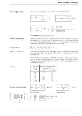
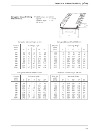
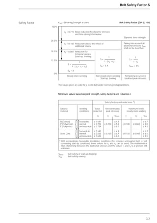
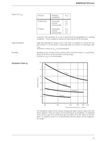
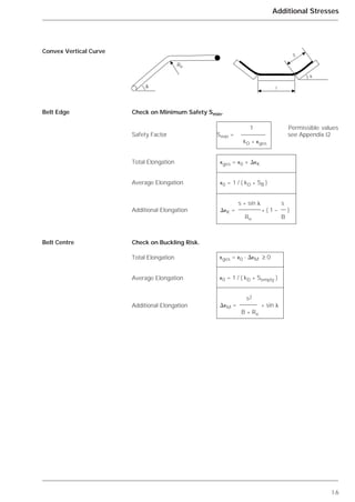
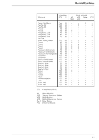
![11.17
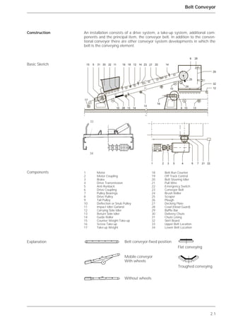
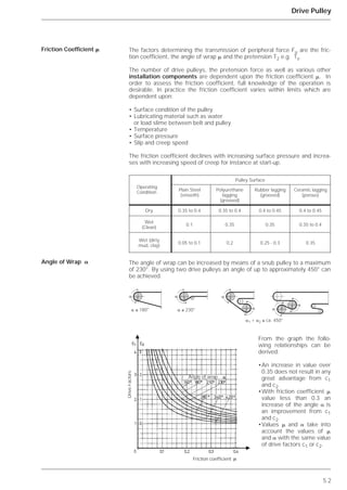
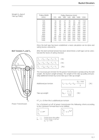
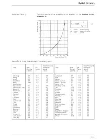
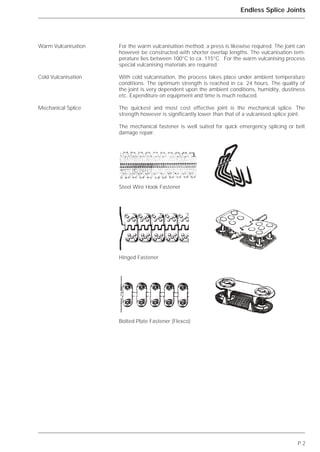
Design
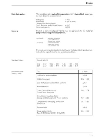
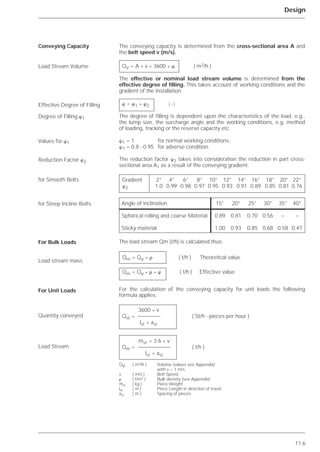
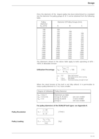
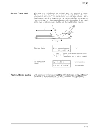
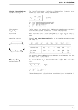
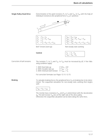
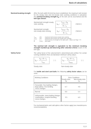
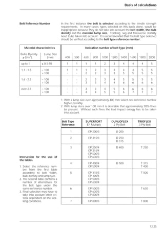
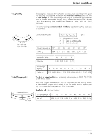
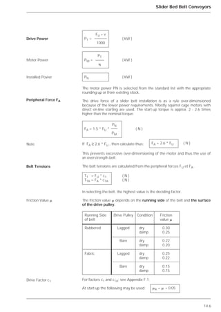
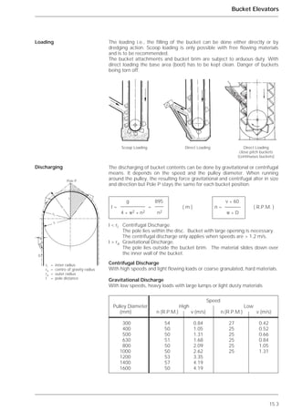
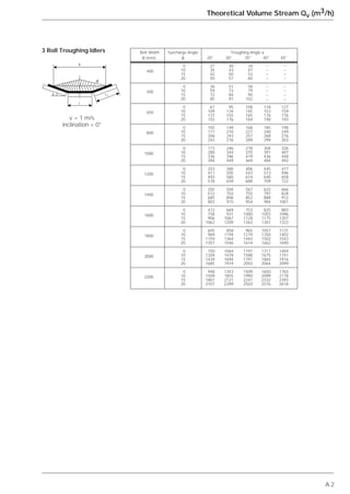
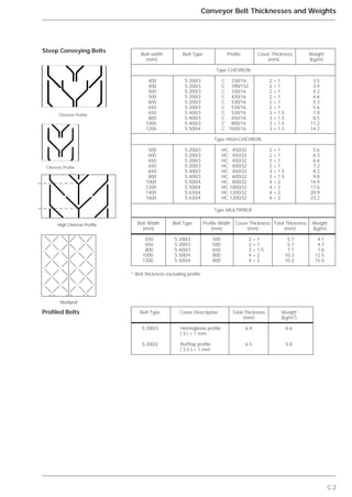
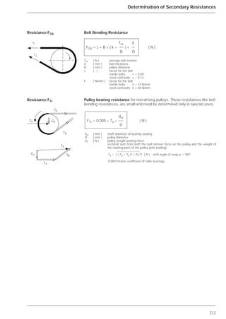
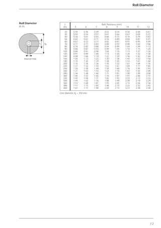
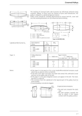
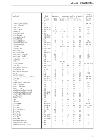
Within limits, belts are able to negotiate horizontal curves. To do this the car-
rying idlers on the inside of the curve are slightly raised by the angle R accor-
ding to radius and belt tension by approximately 5°-15°.
The exact position has to be determined by adjustment.
For design purposes the following radii may be selected being the smaller
permissible radii RH (m).
The values RH apply to a troughing angle of 30°
Horizontal Curve
Value of Curve Radius
RH
᭤
᭤
᭤
RH
R
l
Inside of Curve
l
RH = k * [ l + B * ( 1 - ) * cos ] ( m )
B
l ( mm ) Length of middle carrying roller (see Page 11.3)
B ( mm ) Belt width
( ° ) Troughing angle
R ( ° ) Lifting of the carrying rollers (ca. 5° to 15°)
k ( - ) Factor (consider belt type and duty)
for EP belts k = 71
DUNLOPLAST k = 150
FERROFLEX k = 225
ST belts k = 245
Belt width
(mm) 300 400 500 650 800 1000 1200 1400
EP belts 20 26 33 42 52 65 72 91
DUNLOPLAST 42 56 69 89 110 137 165 192
FERROFLEX - - - 134 165 206 248 289
ST belts - - - 146 180 224 270 314
Belt width
(mm) 1600 1800 2000 2200 2400 2600 2800
EP belts 104 117 130 142 156 169 182
DUNLOPLAST 220 247 275 - - - -
FERROFLEX 329 370 412 452 - - -
ST belts 359 404 449 493 - - -](https://image.slidesharecdn.com/beltconveyordesign-dunlop-140630061205-phpapp02/85/Belt-conveyor-design-dunlop-51-320.jpg)
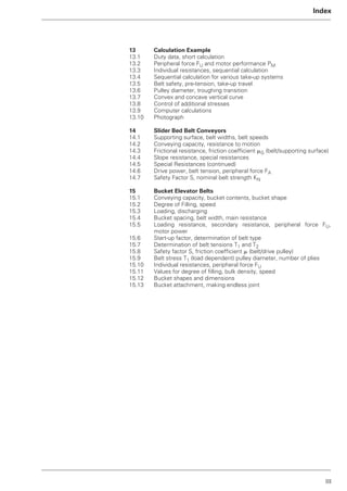
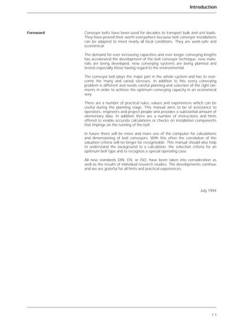
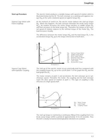
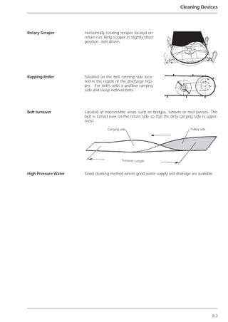
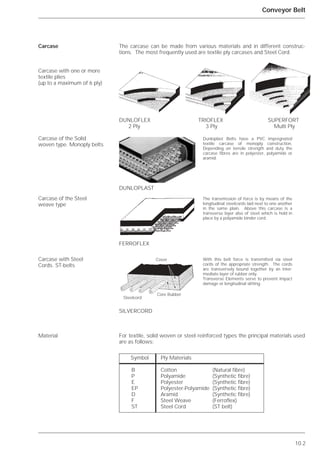
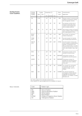
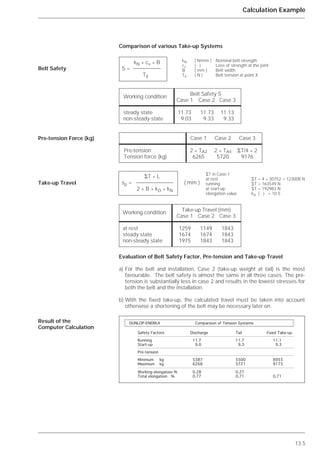
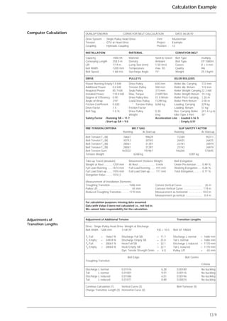
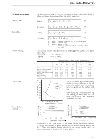
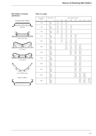
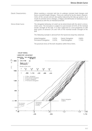
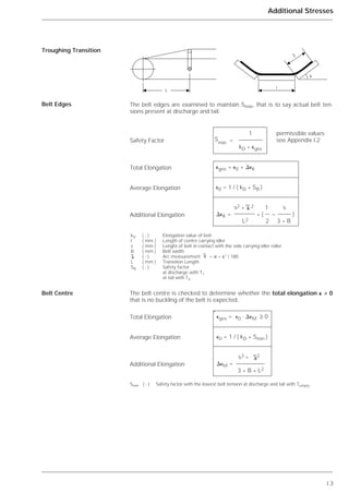
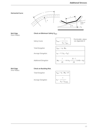
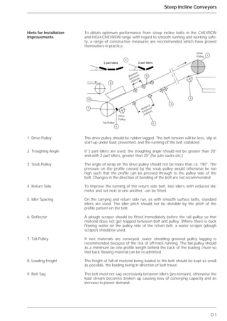
![12.1
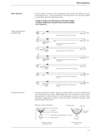
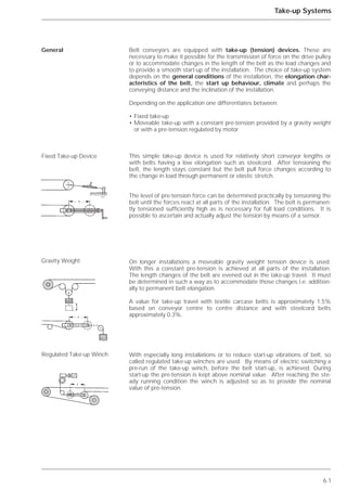
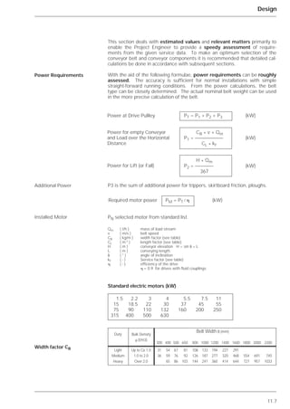
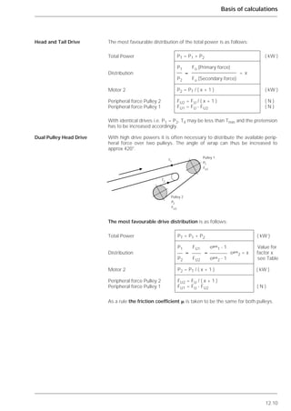
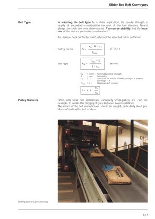
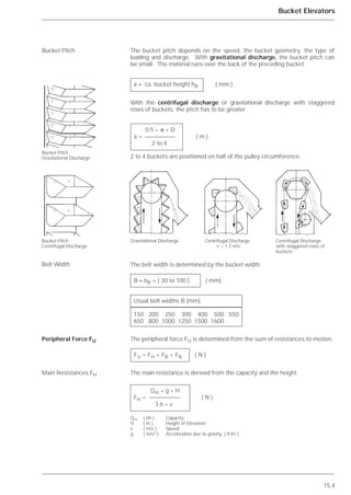
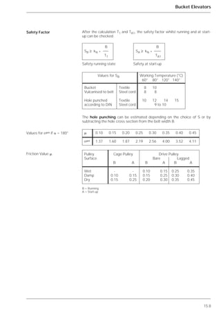
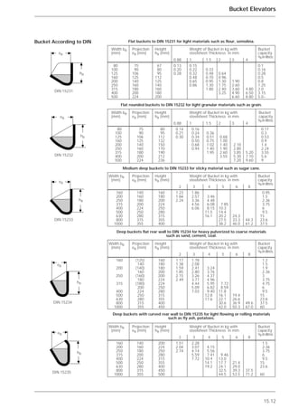
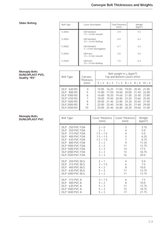
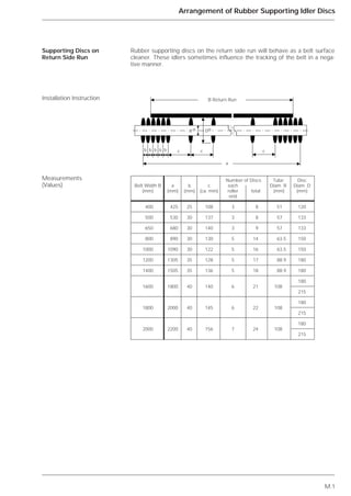
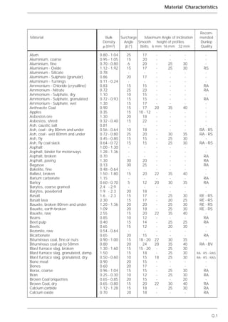
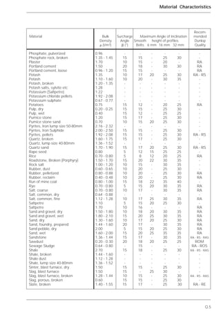
Basis of calculations
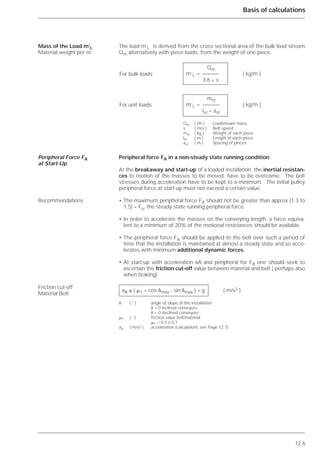
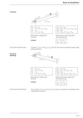
After the design of the installation and the main data has been determined an
exact calculation can be undertaken. Established installation components
can be checked and dimensioned. The belt selection can be undertaken
according to forces that have been established and other relevant
criteria.
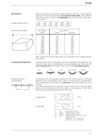
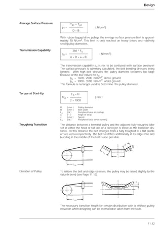
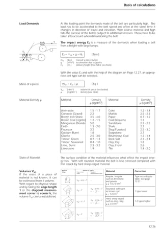
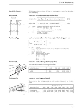
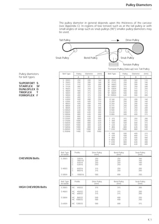
The resistances to motion within a belt installation may be categorised thus:
- Main resistance
- Secondary resistance
- Slope resistance
- Special resistances
Resistance due to moving the mass of idlers, belt and material on the car-
rying and return runs. Running resistance of idlers (bearing and seal fric-
tion). Resistance due to impressions made in the belt by idlers and the
flexing of the belt.
With gradients ␦ ≤ 18° Cos ␦ = 1.
Resistance occurring mainly in the loading area such as the acceleration of
the material at the loading point. Resistance due to the friction on the side
walls of the chute, resistance due to belt flexing on pulleys, pulley bearing
resistance.
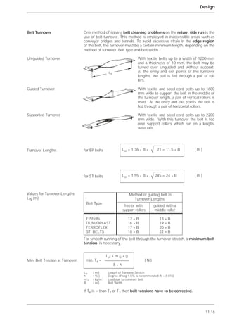
• With normal installations with one loading point, the secondary resistance
can be calculated by using the factor C as part of the main resistance.
Factor C depends on the conveying length and can be taken from the table
on Page 12.3.
• If the secondary resistance relative to the total resistance is high as for
instance with conveyors less than approximately 80 m long with several
loading points, a separate calculation is necessary.
Resistance from load and elevation.
The special resistances are due to installation components such as:
• the forward tilt of outer idler rollers to improve tracking
• material deflection ploughs and belt cleaners, continuous skirtboards
• trippers (throw-off carriages)
• bunker drag out belts
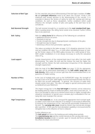
The resistances to motion are relatively simple to calculate. Information not
available such as pulley diameters etc. can be estimated for initial calculation
formulae or taken from the appropriate table.
Formulae for calculation: see Appendix E.
Resistance to Motion FH
Main Resistance FH
Secondary Resistance FN
Note
Slope Resistance FSt
Special Resistances FS
FH = f * L * g * [ m’R + ( 2 * m’G + m’L ) * cos ␦ ] ( N )
FN = ( C - 1 ) * FH ( N )
FSt = H * g * m’L ( N )](https://image.slidesharecdn.com/beltconveyordesign-dunlop-140630061205-phpapp02/85/Belt-conveyor-design-dunlop-52-320.jpg)
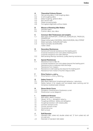
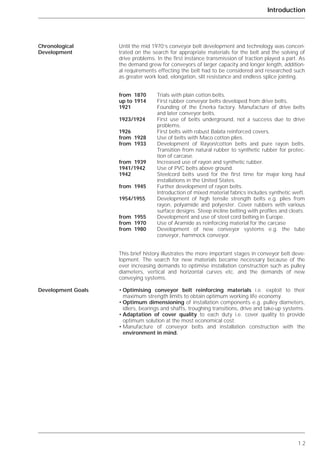
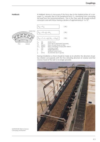
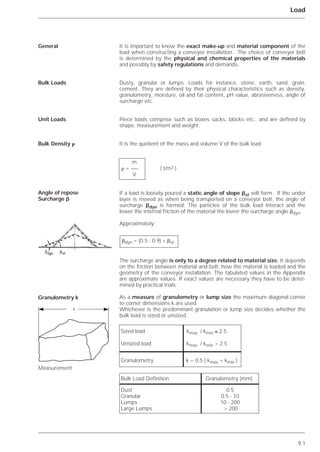
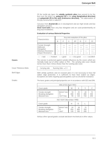
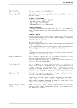
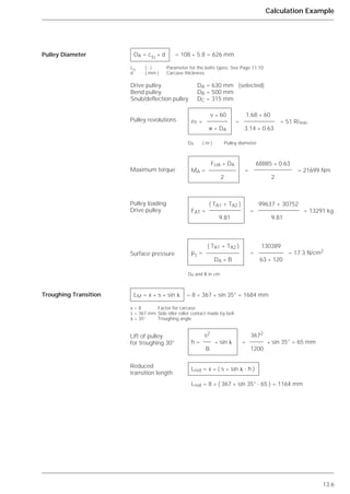
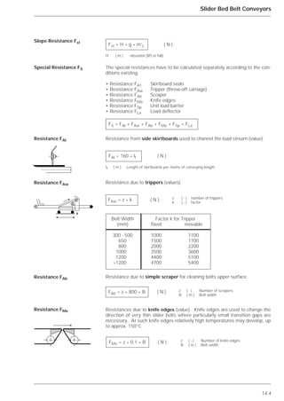
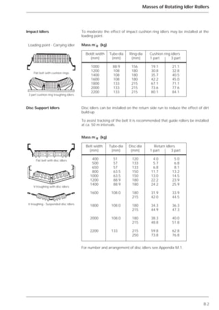
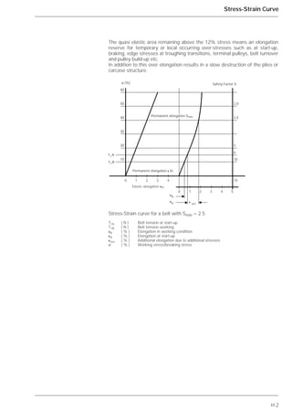
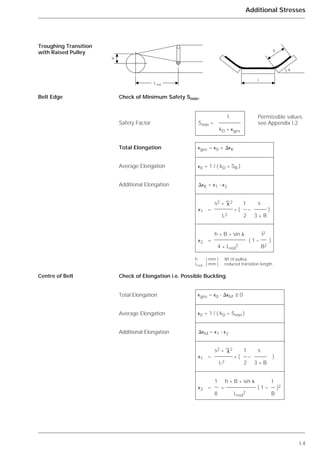
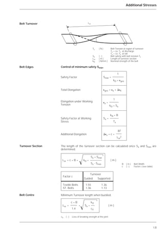
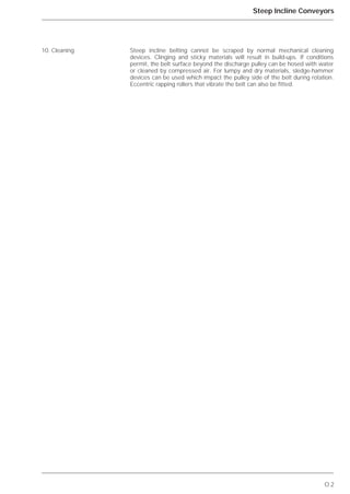
![12.2
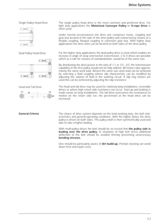
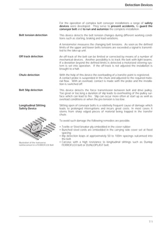
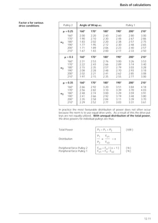
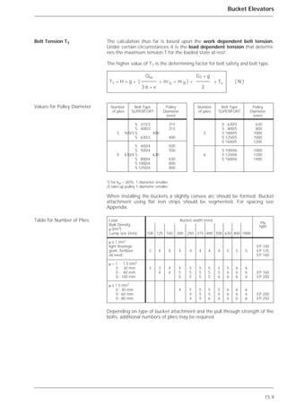
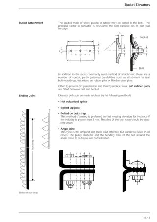
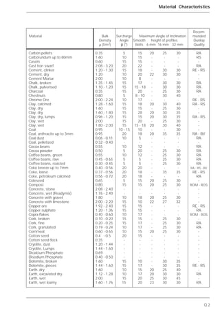
Basis of calculations
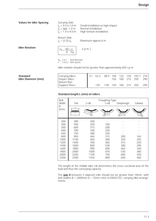
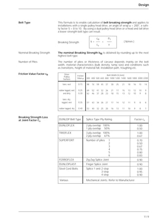
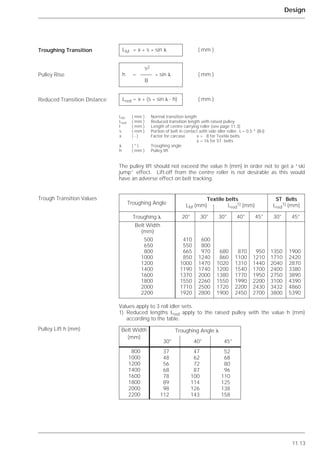
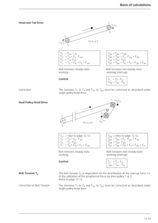
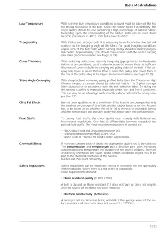
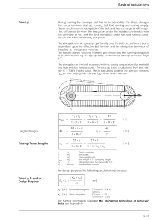
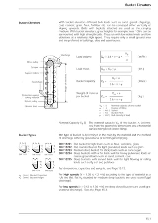
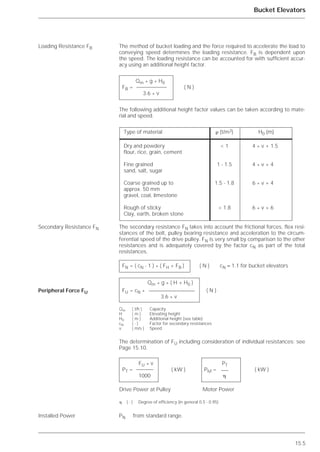
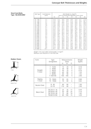
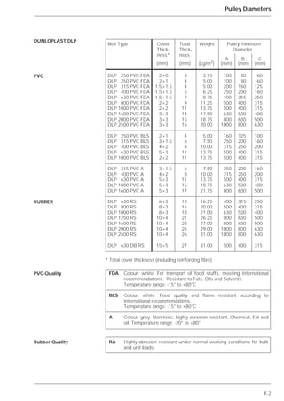
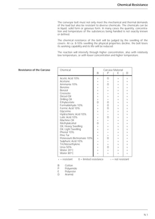
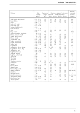
Peripheral force steady state working
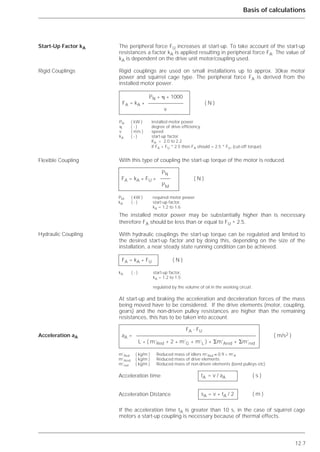
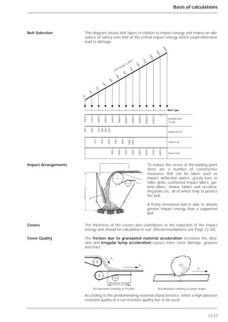
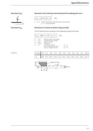
The sum of the resistances to motion is equal to the peripheral force FU at
the drive pulley (or shared over several drive pulleys).
For installations with one loading point, as a rule the following summation
applies:
Peripheral Force FU
Working Conditions
Summation
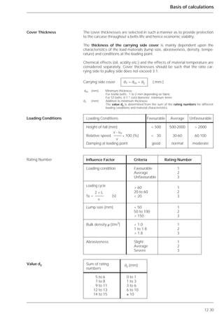
Herringbone Belt in Operation
FU = FH + FN + FSt + FS ( N )
FU = C * f * L * g * [m’R + (2 * m’G + m’L) * cos ␦] + H * g * m’L + FS ( N )
C ( - ) Length factor
f ( - ) Artificial friction factor
L ( m ) Conveyor length
g ( m/s2 ) Acceleration due to gravity
m’R ( kg/m ) Mass of the rotating carrying and return idlers
m’G ( kg/m ) Mass of the belt
m’L ( kg/m ) Mass of the load
␦ ( ° ) Gradient of the installation with ␦ ≤ 18° cos ␦ = 1
H ( m ) Conveying height
H > 0 inclined conveying
H < 0 declined conveying
FS ( N ) Sum of the special resistances. For separate calculations see Appendix.](https://image.slidesharecdn.com/beltconveyordesign-dunlop-140630061205-phpapp02/85/Belt-conveyor-design-dunlop-53-320.jpg)
![13.2
Calculation Example
Peripheral Force
Peripheral Force
FU = C * f * L * g [ m’R + ( 2 * m’G + m’L ) * cos ␦ ] + H * g * m’L
Factor C = 1.37
Friction factor f = 0.02
Drive Power and Belt Tension
22.3 19.3
m’R = + = 18.6 + 9.6 = 28.2 kg/m
1.2 2
m’G = 25.4 kg/m
1000
m’L = = 165.3 kg/m
3.6 * 1.68
␦ = 4.8° cos 4.8° = 0.997
kA = 1.5 (hydraulic coupling)
FU = 16897 + 29027 = 45924 N
FA = 45924 * 1.5 = 68885 N
45923 * 1.68
PT = = 77.2 kW
1000
drive degree of efficiency = 0.9
PT
PM = = 85.7 kW
0.9
PN = 110 kW (selected)
( m’L + m’G ) * g * lo
Tmin = = 28061 N
8 * 0.01
With belt sag 1%
Carrying side idle pitch lo = 1.2m
68885 - 45924
aA = = 0.368 m/s2
258 * ( 165.3 + 25.4 + 50.8 )
1.68
tA = = 4.56 s
0.368
1.68 * 4.56
sA = = 3.83 m
2
Load due to idlers
Load due to belt
Load due to material
Incline
Start-up factor
Steady state
Non-steady state
Power at pulley
Motor power
Installed motor power
Min. belt tension
Acceleration
Start-up time
Start-up distance
FU = 1.37*0.02*258*9.81[28.2+(2*25.4+165.3)*0.997]+17.9*9.81*165.3](https://image.slidesharecdn.com/beltconveyordesign-dunlop-140630061205-phpapp02/85/Belt-conveyor-design-dunlop-84-320.jpg)
![13.3
Calculation Example
Individual Resistances for Sequential Calculation
Case 1) Tension Weight at Discharge Point (close to T2)
TA2 = T2 (constant tension)
⌬T = TA2 - T2 = 26424 - 22961 = 3463 N
With the value ⌬ T belt tensions T1 to T4 are increased
T1 = 72347 N TA1 = 95309 N
T2 = 26424 N TA2 = 26424 N
T3 = 23732 N TA3 = 26969 N
T4 = 23732 N TA4 = 26969 N
Tmin = 28061 N est nécessaire pour la flèche de 1%, i.e. T4 ≥ Tmin
⌬T = Tmin - T4 = 28061 - 23732 = 4328 N
With the value ⌬ T all belt tensions T1 to T4 and TA1 to TA4 will be increased
Main resistance
Secondary resistance
Frictional Resistances
Carrying side
Return side
Slope Resistance
Carrying side
Return side
Inertial Resistance
Carrying side
Return side
Running (steady state)
Control T1
Start-up (non-steady state)
Control TA1
1st Adjustment
2nd Adjustment
Belt Tensions
FH = 0.02 * 258 * 9.81 * [ 28.2 + ( 50.8 + 165.3 ) * 0.997 ] = 12333 N
FN = ( C - 1 ) * FH = 12333 * 0.37 = 4563 N
Fo = 0.02 * 258 * 9.81 * [ 18.6 + ( 25.4 + 165.3 ) * 0.997 ] = 10566 N
Fu = 0.02 * 258 * 9.81 * ( 9.6 + 25.4 ) * 0.997 = 1768 N
Fsto = 17.9 * 9.81 * ( 25.4 + 165.3 ) = 33486 N
Fstu = 17.9 * 9.81 * 25.4 = 4460 N
Fao = 0.368 * 258 * ( 16.7 + 25.4 + 165.3 ) = 19725 N
Fau = 0.368 * 258 * ( 8.7 + 25.4 ) = 3237 N
Sequential Calculation T1 to T4
T2 = FU * c2 = 45924 * 0.5 = 22961 N
T3 = 22962 + 1768 - 4460 = 20269 N
T4 = T3 = 20269 N
T1 = 20269 + 4563 + 10566 + 33486 = 68884 N
Sum = 132383 N
T1 = FU * c1 = 45924 * 1.5 = 68884 N
TA2 = FA * c2A = 68886 * 0.3836 = 26424 N
TA3 = 26424 + 1768 - 4460 + 3237 = 26969 N
TA4 = TA3 = 26969 N
TA1 = 26969 + 4563 + 10566 + 33486 + 19725 = 95309 N
Sum = 175671 N
TA1 = FA * c1A = 68886 * 1.3836 = 95309 N
T1 = 76675 N TA1 = 99637 N
T2 = 30752 N TA2 = 30752 N
T3 = 28061 N TA3 = 31297 N
T4 = 28061 N TA4 = 31297 N
⌺T = 163549 N ⌺TA = 192983 N
The stipulations T2 = TA2 and T4 ≥ Tmin are fulfilled.](https://image.slidesharecdn.com/beltconveyordesign-dunlop-140630061205-phpapp02/85/Belt-conveyor-design-dunlop-85-320.jpg)


This document provides an overview of conveyor belt techniques, including: - A brief history of conveyor belt development from the late 19th century to present day. Key milestones included the introduction of rubber belts, steel cord belts, and new reinforcing materials. - The document aims to assist operators, engineers, and project managers by providing elementary data, instructions, and tips for accurate calculations and component selection. - It covers topics like belt and drive system design, belt materials, calculations, installation examples, and more. The goal is to help understand the background and criteria for optimizing belt and conveyor system selection.


