This document provides information about a finite element method course, including:
- The course covers basic knowledge and skills for understanding and applying the finite element method.
- Lectures will cover topics like introductions to FEM, various applications, finite difference methods, boundary element methods, beams, bars, trusses, frames, and elements.
- Laboratories will involve modeling practical problems in ANSYS and conducting static analyses of structures.
- Upon completing the course, students will be able to build simple FEM models and understand applications and limitations of the method.
![Page 1 of 89
_________________________________________________________________________________________________________________________________________________________________________
Course Title: FINITE ELEMENT METHOD I
Type of course: undergraduate, graduate
Field of study (Programme), specialization
Aerospace Engineering, Power Engineering, Robotics, Computer Aided Engineering
Format
(Teaching methods)
Lectures:
2hours/week
Laboratory:
1hour/week
Private study:
2hours/week
Lecturers (course leader): Grzegorz Krzesiński
Objective: To supply the basic knowledge and skills required for understanding and simple practical applications of FEM
Contents (lecture’s programme):
1. INTRODUCTION TO FINITE ELEMENT METHOD
2. APPLICATIONS OF FEM
3. FINITE DIFFERENCE METHOD (FDM), BOUNDARY ELEMENT METHOD (BEM) AND FINITE ELEMENT METHOD (FEM)
4. BEAMS. RITZ-RAYLAYGH METHOD and FINITE ELEMENT METHOD
5. BARS AND SPRINGS
6. TRUSSES AND FRAMES
7. TWO AND THREE- DIMENSIONAL LINEAR ELASTOSTATICS
8. CST TRIANGULAR ELEMENT
9. 8-NODE QUADRILATERAL ELEMENT . NUMERICAL INTEGRATION
Computer lab: Introduction to practical problems of FE modeling in ANSYS/ 2D and 3D linear stress analysis/ Static analysis of simple shell structure/
Discretization error and adaptive meshing
Abilities: After completing the course the students will be able to build simple FE models and will know the possible applications and
limitations of the method in mechanics of structures.
Assesment method: Assesment based on tests and results of computer lab work (reports).
Practical work:Project/laboratory classes, where students will build and analyse the results of simple FE models of elastic structures
Recommended texts (reading):
[1] Huebner K. H., Dewhirst D. L., Smith D.E., Byrom T. G.: The finite element method for engineers, J. Wiley & Sons, Inc., 2001.
[2] Zagrajek T., Krzesinski G., Marek P.: MES w mechanice konstrukcji. Ćwiczenia z zastosowaniem programu ANSYS, Of.Wyd.PW 2005
[3] Bijak-Żochowski M., Jaworski A., Krzesiński G., Zagrajek T.: Mechanika Materiałów i Konstrukcji, Tom 2, Warszawa, Of. Wyd. PW, 2005
[4] Saeed Moaveni: Finite Element Analysis. Theory and Application with ANSYS, Paerson Ed. 2003
[5] Cook R. D.: Finite Element Modeling for Stress Analysis, John Wiley & Sons , 1995
[6] Zienkiewicz O.C., Taylor R.: The Finite Element Method.- different publishers and editions](https://image.slidesharecdn.com/finiteelementmethodilecturenotes-240221175018-b484efa5/85/FINITE-ELEMENT-METHOD-I-lecture-notes-pdf-1-320.jpg)


![Page 22 of 89
_________________________________________________________________________________________________________________________________________________________________________
Differences corresponding to higher derivatives
2 2
1, , 1,
2 2 2
2 2
, 1 , , 1
2 2 2
2
,
2
.
i k i k i k
i k i k i k
u u u
u u
x x h
u u u
u u
y y g
+ −
+ −
− +
∂ ∆
≈ =
∂ ∆
− +
∂ ∆
≈ =
∂ ∆
Using the finite differences we can approximate the partial differential equation at any point (xi, yj ) by an algebraic equation .
In the case of Poissons equation:
( ) ( ) ( )
1, , 1, , 1 , , 1
2 2
1 1
2 2 , 0
i j i j i j i j i j i j i j
u u u u u u f x y
h g
+ − + −
− + + − + + = .
If h g
= i 0
f ≡ (Laplace equation) we get
1, 1, , 1 , 1
,
4
i j i j i j i j
i j
u u u u
u
+ − + −
+ + +
= .
N grid points in the domain Ω , N equations, N unknows
[ ]{ } { }
A u b
=
discrete form of boundary conditions
1
2 0 1
2 0
h
h
δ
δ
a) b)
In the case of irregular boundary shape
a) assumed 0 2
1
hu u
u
h
δ
δ
+
=
+
instead of 0
u u
=
b) assumed 0 2
1
hu u
u
h
δ
δ
−
=
−
instead of 0
u u
=
4 4
2, 1, , 1, 2,
4 4 4
4 6 4
i j i j i j i j i j
u u u u u
u u
x x h
+ + − −
− + − +
∂ ∆
≈ =
∂ ∆](https://image.slidesharecdn.com/finiteelementmethodilecturenotes-240221175018-b484efa5/85/FINITE-ELEMENT-METHOD-I-lecture-notes-pdf-22-320.jpg)


![Page 25 of 89
_________________________________________________________________________________________________________________________________________________________________________
The numerical approach
1. Discretization of the boundary (LE boundary elements)
2. Approximation of ( )
u x and ( )
q x on the boundary
(e.g. u(Pi), q(Pi) constant on boundary elements)
3 . Building the set of linear equations
1 1
1
( ) ( , ) ( ) ( , ) ( )
2
( ) ( , ) 1,2,..
j j
LE LE
i i j j i j j
j j
i
u P u P x q P d q P x u P d
f x u P x dR i LE
∗ ∗
= =
Γ Γ
∗
Ω
= Γ − Γ
+ =
∑ ∑
∫ ∫
∫
1 1
1
( ) ( ) ( ) , 1,2...
2
LE LE
i ij j ij j i
j j
u P U q P Q u P f i LE
∗ ∗
= =
= ⋅ − ⋅ + =
∑ ∑ . ( ) ( , ) ( )
i i
f f x u P x d x
∗
Ω
= Ω
∫
{ } { } { } { }
1
2
u U q Q u f
∗ ∗
= − +
.
LE linear equations with the unknows ( )
j
u P (if the point j
P Πq
Γ ) or ( )
i
q P (if i
P Πu
Γ )
Finally: [ ]{ } { }
A y b
=
The solution {y} represents unknown boundary values of u and q.
The matrix A – full, unsymmetric
4. Solution - provides complete information about the function ( )
u x and its derivative ( )
q x on the boundary
Boundary Element Method reduces the number of unknown parameters (DOF of the discrete model) in comparison to FDM and FEM ( domain
methods).
x
x2
1
P
P
j
i
r](https://image.slidesharecdn.com/finiteelementmethodilecturenotes-240221175018-b484efa5/85/FINITE-ELEMENT-METHOD-I-lecture-notes-pdf-25-320.jpg)

![Page 27 of 89
_________________________________________________________________________________________________________________________________________________________________________
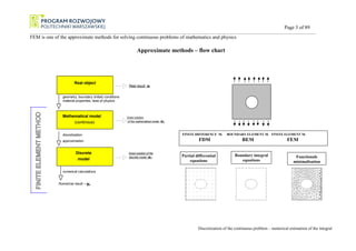
In each element
1
1 1
1
2 2
,
.
LWE
i
i
i
LWE
i
i
i
N
u
u
x x
N
u
u
x x
=
=
∂
∂
=
∂ ∂
∂
∂
=
∂ ∂
∑
∑
In this way the functional I is replaced by the function of several unknows , 1,2,...,
i
u i LW
= , where LW denotes the number of nodes of the finite
element mesh. In the matrix form :
11 12 13 1 1 1
21 22 23 2 2
31 32
1 2 3 1 2 3,
3 3
1
1
( ) , , ,..., , , ,
2
LW
LW LW
LW LW LW LW LW
k k k k u b
k k k u b
k k
I u u u u u u u u u
u b
k k u b
≈ −
…
…
… … …
[ ]{ } { }
1 1
1 1
1
2 LW LW
LW LW
LW LW
I u u u b
K
× ×
× ×
×
≈ −
.
Necessary (and sufficient) condition of the minimum:
0
i
I
u
∂
=
∂
, 1, ,
i LW
= … . matrix: sparse, symmetrical, positive defined, banded
Hence
[ ]{ } { }
K u b
= , (+ Dirichlet b.c.)
Set of the simultaneuous equations with unknown nodal values of the investigated function.
zerowe
elementy
LW
m](https://image.slidesharecdn.com/finiteelementmethodilecturenotes-240221175018-b484efa5/85/FINITE-ELEMENT-METHOD-I-lecture-notes-pdf-27-320.jpg)

![Page 29 of 89
_________________________________________________________________________________________________________________________________________________________________________
Total potential energy of the beam loaded by the distributed load
N
m
p
:
2
0 0
1
( )
2
l l
V EI w dx pwdx
′′
= −
∫ ∫ ,
where the function w(x) describes deflection of the beam
Ritz method
3. The parameters ai are determined by requirement that the
functional is minimized with respect to ai
0
i
V
a
∂
=
∂
, 1,...,
i n
= .
[ ]{ } { }
A a b
=
4. The solution provides ai, and the approximate solution
1
( ) ( )
n
i i
i
w x a x
ϕ
=
= ∑
ɶ .
Hence the approximate internal forces in the beam
( ) ( ),
( ) ( ).
q
M x EIw x
T x EIw x
′′
=
′′′
= −
ɶ ɶ
ɶ ɶ
1.The problem must be stated in a variational form,
as a minimization problem, that is:
find w(x) minimizing the functional V(w)
2. The solution is approximated by a finite linear combination of the
form:
1
( ) ( )
n
i i
i
w x a x
ϕ
=
= ∑
ɶ
where ai denote the undetermined parameters termed Ritz
coefficients,
and φi are the assumed approximation functions (i=1,2...n).
The approximate functions φi must be linearly independent
and
3. Finally functional V is approximated by the function of n variables
ai
V=V(a1, a2 , a3 , ....an )](https://image.slidesharecdn.com/finiteelementmethodilecturenotes-240221175018-b484efa5/85/FINITE-ELEMENT-METHOD-I-lecture-notes-pdf-29-320.jpg)


![Page 35 of 89
_________________________________________________________________________________________________________________________________________________________________________
{ } { }
0 0
1 1 1 2 1 3 1 4
2 1 2 2 2 3 2 4
3 1 3 2 3 3 3 4
4 1 4 2 4 3 4 4
( ) ( )
2 2
2
e e
l l
e e
e
e
EI EI
U w w d q N N q d
N N N N N N N N
N N N N N N N N
EI
q
N N N N N N N N
N N N N N N N N
ξ ξ ξ ξ
′′ ′′ ′′ ′′
= = =
′′ ′′ ′′ ′′ ′′ ′′ ′′ ′′
′′ ′′ ′′ ′′ ′′ ′′ ′′ ′′
=
′′ ′′ ′′ ′′ ′′ ′′ ′′ ′′
′′ ′′ ′′ ′′ ′′ ′′ ′′ ′′
∫ ∫
{ }
0
.
e
l
e
d q
ξ
∫
[ ] { }
1
2
e e
e e
U q k q
=
,
.
Matrix [ ]e
k is named stiffness matrix of beam element. After integration
[ ]
2 2
3
2 2
6 3 6 3
3 2 3
2
6 3 6 3
3 3 2
e e
e e e e
e
e e
e
e e e e
l l
l l l l
EI
k
l l
l
l l l l
−
−
=
− − −
−
.
[ ]
1 1 1 2 1 3 1 4
0 0 0 0
2 1 2 2 2 3 2 4
0 0 0 0
3 1 3 2 3 3 3 4
0 0 0 0
4 1 4 2
0 0
e e e e
e e e e
e e e e
e e
l l l l
l l l l
e l l l l
l l
N N d N N d N N d N N d
N N d N N d N N d N N d
k EI
N N d N N d N N d N N d
N N d N N d
ξ ξ ξ ξ
ξ ξ ξ ξ
ξ ξ ξ ξ
ξ ξ
′′ ′′ ′′ ′′ ′′ ′′ ′′ ′′
′′ ′′ ′′ ′′ ′′ ′′ ′′ ′′
=
′′ ′′ ′′ ′′ ′′ ′′ ′′ ′′
′′ ′′ ′′ ′′
∫ ∫ ∫ ∫
∫ ∫ ∫ ∫
∫ ∫ ∫ ∫
∫ 4 3 4 4
0 0
e e
l l
N N d N N d
ξ ξ
′′ ′′ ′′ ′′
∫ ∫ ∫](https://image.slidesharecdn.com/finiteelementmethodilecturenotes-240221175018-b484efa5/85/FINITE-ELEMENT-METHOD-I-lecture-notes-pdf-35-320.jpg)
![Page 36 of 89
_________________________________________________________________________________________________________________________________________________________________________
The external work done by the traction p:
{ }
0 0
( ) ( ) ( ) ( )
e e
l l
p
ze e
W p w d p N q d
ξ ξ ξ ξ ξ ξ
= = =
∫ ∫ { }
1 2 3 4
0
( ) ( ) , ( ) ( ) , ( ) ( ) , ( ) ( ) ,
e
l
e
N p d N p d N p d N p d q d
ξ ξ ξ ξ ξ ξ ξ ξ ξ ξ ξ ξ ξ
=
∫
{ }
1
2
1 2 3 4
3
4
, , ,
p e e e e
ze e
e
e
q
q
W F F F F F q
q
q
= =
,
0
( ) ( )
e
l
e
i i
F N p d
ξ ξ ξ
= ∫
e
i
F - equivalent nodal forces
0
1 3
2
0
2
2
0
4
2
12
12
e e e
e e
e e
p l
F F
p l
F
p l
F
= =
=
−
=
Equivalent nodal forces corresponding to the constant and linear distribution of 0
p load
(kinematically equivalent or work-equivalent !)
Total potential energy of the beam element
[ ] { } { }
4 4 4 1
1 4 1 4
4 1
1
2
e e ze
V U W q q q F
k e e
e e
e
× ×
× ×
×
= − = − .
1 2
0
p
p
2
0 e 0 e
2
0 e
12
2
12
2
e
0
p
p
p
P0
1 2
F1=3p0 le/ 20 F3= 7p0 le/ 20
F2=p0 le
2
/ 30 F4= -p0 le
2
/ 20](https://image.slidesharecdn.com/finiteelementmethodilecturenotes-240221175018-b484efa5/85/FINITE-ELEMENT-METHOD-I-lecture-notes-pdf-36-320.jpg)
![Page 37 of 89
_________________________________________________________________________________________________________________________________________________________________________
The conditions for finding the minimum of Ve:
0
e
i
V
q
∂
=
∂ , 1,2,3, ,
i n
= …
[ ] { } { }
e e e
k q F
= .
1 1
2 2
2 2
3
3 3
2 2
4 4
6 3 6 3
3 2 3
2
6 3 6 3
3 3 2
e e
e e e e
e e
e
e e
e e e e
l l q F
q F
l l l l
EI
q F
l l
l
q F
l l l l
−
−
=
− − −
−
Set of linear equations for one element model of the considered cantilever beam:](https://image.slidesharecdn.com/finiteelementmethodilecturenotes-240221175018-b484efa5/85/FINITE-ELEMENT-METHOD-I-lecture-notes-pdf-37-320.jpg)
![Page 38 of 89
_________________________________________________________________________________________________________________________________________________________________________
1
2
2 2
0
3
3
2 2 2
4 0
0
6 3 6 3
0
3 2 3
2
6 3 6 3 2
3 3 2
12
F
l l F
l l l l
EI p l
q
l l
l
q
l l l l p l
−
−
=
− − −
− −
Constraints q1=0 and q2=0 may be taken into account by
the transformation of the set of equation to the form [ ] { }
1
2
3
4
F
F
A b
q
q
=
or by reductionof the problem to
0
3 4
3
2
2 0
3 4
3
2
(6 3 ) ,
2
2
( 3 2 ) ,
12
p l
EI
q lq
l
p l
EI
lq l q
l
− =
−
− + =
Solution is:
4
0
3
3
0
4
1
8
1
6
p l
q
EI
p l
q
EI
=
=
Finally the deflection function from the one element model is
2 2
2 3 2 3
0 0 0 0
3 1 2 1 5
( )
8 6 8 6 24 12
p l p l p l p l
w
EI EI EI EI
ξ ξ ξ ξ ξ
−
= − + + = −
The same result as obtained in the case of Ritz method – why?](https://image.slidesharecdn.com/finiteelementmethodilecturenotes-240221175018-b484efa5/85/FINITE-ELEMENT-METHOD-I-lecture-notes-pdf-38-320.jpg)
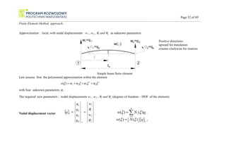
![Page 39 of 89
_________________________________________________________________________________________________________________________________________________________________________
Dividing the beam into LE elements
global nodal displacements vector { }
1 1
2 1
3 2
4 2
5 3
6 3
7 4
8 4
q w
q
q w
q
q
q w
q
q w
q
θ
θ
θ
θ
= =
.
N=8 nodal diplacements (degrees of freedom of the FE model)
Strain energy e
U of each of the elements
[ ] { }
1
2
e e e
e
U q k q
=
[ ]{ }
*
1
1
1
2
e
N N N
N e
q q
k
× ×
×
= ,
1
k∗
=
2
k∗
=
3
k∗
=
1 2
0
p
3 4
P
M
1 2 3
1
q q3
q5
q7
q2 4
q q6
q8
=
3
e
e e e
1x4 4x4 4x1
element 1 with the global DOF :
q1, q2 , q3, q4
element 2 with the global DOF :
q3, q4 , q5, q6
element 3 with the global DOF :
q5, q6 , q7, q8](https://image.slidesharecdn.com/finiteelementmethodilecturenotes-240221175018-b484efa5/85/FINITE-ELEMENT-METHOD-I-lecture-notes-pdf-39-320.jpg)
![Page 40 of 89
_________________________________________________________________________________________________________________________________________________________________________
{ } [ ]{ }
1 1
1 1
2 2
LE LE
e e
e i
U U q k q q K q
∗
= =
= = =
∑ ∑ .
[ ]{ } { }
1
2
z
V U W q K q q F
= − = −
,
0
i
V
q
∂
=
∂ , 1,2,3, ,
i n
= …
[ ]{ } { }
K q F
= . + displacement boundary conditions (constraints)
For each element the internal forces M,T are calculated separately:
1
2
1 2 3 4
3
4
1
2
1 2 3 4
3
4
( ) ( ) , , , ,
( ) ( ) , , , .
q
e
e
q
q
M EIw EI N N N N
q
q
q
q
T EIw EI N N N N
q
q
ξ ξ
ξ ξ
′′ ′′ ′′ ′′
′′
= =
′′′ ′′′ ′′′ ′′′
′′′
= − =
1 2 3 4
3 2 3 2
1 3 2 4
3 2
12 6 2 12 6
( ) ( ) ( ) ( ) ( ) ,
2 3 2 3
12 6
( ) ( ) ( ) .
e e e
q e
e e e e
e e
l l l
M q l q q q EI
l l l l
T q q q q EI
l l
ξ ξ ξ ξ ξ
ξ
= − + − − − + −
= − − + +
](https://image.slidesharecdn.com/finiteelementmethodilecturenotes-240221175018-b484efa5/85/FINITE-ELEMENT-METHOD-I-lecture-notes-pdf-40-320.jpg)

![Page 42 of 89
_________________________________________________________________________________________________________________________________________________________________________
FEM calculations:
1. Generation of stiffness matrices [ ]e
k for all elements
2. Assembling the element matrices to obtain the global stiffness matrix [ ]
K
3. Finding the equivalent nodal force vector { }
F
4. Imposing the boundary conditions and the solution of the final set of linear equations – finding all nodal displacements { }
q
5. Calculation of the internal forces (bending moment, shear force) and the stresses within the elements
The example
Final set of equations (3 active DOF)
3
2 2
4 1
3
2 2
6 2
12 0 3
2
0 4
3 2
l q P
EI
l l q M
l
l l l q M
−
=
.
2
3 2
4 2 1
6 3 2
7 3 12
3 15 12
96
12 12 48
q w l l l P
l
q l M
EI
q l M
θ
θ
− −
= = −
− −
.
(exact solution – why?)
4x4
NxN
Nx1
Nx1
1
2
2 3
P
M
1
M
1 2
A B C](https://image.slidesharecdn.com/finiteelementmethodilecturenotes-240221175018-b484efa5/85/FINITE-ELEMENT-METHOD-I-lecture-notes-pdf-42-320.jpg)

![Page 44 of 89
_________________________________________________________________________________________________________________________________________________________________________
Strain energy of the element:
2
0 0
1
( ) ( ) ( ( ))
2 2
e e
l l
e
EA
U A d d
σ ξ ε ξ ξ ε ξ ξ
= =
∫ ∫ .
Taking into account that
1
1 2
2
( ) , .
e
q
du
N N
q
d
ε ξ
ξ
′ ′
= =
we have
[ ] { }
1 1
1 2 1 2
2
0
2
1 1 1 2 1
1 2
2
0
2 1 2 2
, ,
2
1
, ,
2 2
e
e
l
e e
e
l
e
e e e
e
N q
EA
U q q N N d
q
N
N N N N q
EA
q q d q k q
q
N N N N
ξ
ξ
′
′ ′
= =
′
′ ′ ′ ′
= =
′ ′ ′ ′
∫
∫
where
[ ]
1 1
1 1
e
e
EA
k
l
−
=
−
,
is the stiffness matrix of the rod element (symmetric, singular, positive semidefinite)](https://image.slidesharecdn.com/finiteelementmethodilecturenotes-240221175018-b484efa5/85/FINITE-ELEMENT-METHOD-I-lecture-notes-pdf-44-320.jpg)
![Page 45 of 89
_________________________________________________________________________________________________________________________________________________________________________
Equivalent nodal forces
The forces equivalent to the distributed load
N
( )
m
p ξ
.
1
1 2
2
0 0
1
1 2
2
0 0
( ) ( ) ( ) ( ), ( ) ( )
( ) ( ), ( ) ( ) .
e e
e e
l l
p
ze
e
l l
e
q
W p u d N p N p d
q
q
N p N p d
q
ξ ξ ξ ξ ξ ξ ξ ξ
ξ ξ ξ ξ ξ
= = =
=
∫ ∫
∫ ∫
In result:
1
1 2
2
,
p e e
ze e
e
q
W F F
q
=
, where
0
( ) ( )
e
l
e
i i
F N p d
ξ ξ ξ
= ∫ ,
e
i
F - the nodal forces equivalent to the distributed load p (‘work-equivalent’ or ‘kinematically’ equivalent)
Next steps of FE modelling are similar as in the case of the beam element. Finally we get the system of linear quations :
{ } { }
[ ]
K q F
= .
The right side vector { }
F contains the external forces acting on nodes of the model (active nodes and reactions).
The system is solved after taking into account all boundary conditions;
When the vector of nodal displacements is determined the stresses within each of elements are computed:
1 2 1
1 2
2
( )
( ), ( )
e
e
q E q q
E E N N
q l
σ ε ξ ξ
−
′ ′
= = =
.
Example.](https://image.slidesharecdn.com/finiteelementmethodilecturenotes-240221175018-b484efa5/85/FINITE-ELEMENT-METHOD-I-lecture-notes-pdf-45-320.jpg)
![Page 46 of 89
_________________________________________________________________________________________________________________________________________________________________________
Solve the presented below rods using FE models consisted of 2 elements
a
1
1
q =0
2
q2
3
q =0
3
1 2
a
P
P
p0
1
1
q =0
1
2
0
2
p (l-a)
3
q =0
2
2
a) b)
Stiffness matrices of the two finite elements
[ ]
1 1 1
1 1
e
EA
k
a
−
=
−
[ ]
2 1 1
1 1
e
EA
k
l a
−
=
−
−
.
System of simultaneous linear equations
.
After including the boundary conditions 1 3 0
q q
= = and 2
F P
= (case a) we have
1 1
2 2
3 3
1 1
0
1 1 1 1
1 1
a a q F
EA q F
a a l a l a
q F
l a l a
−
− + − =
− −
−
− −
](https://image.slidesharecdn.com/finiteelementmethodilecturenotes-240221175018-b484efa5/85/FINITE-ELEMENT-METHOD-I-lecture-notes-pdf-46-320.jpg)

![Page 48 of 89
_________________________________________________________________________________________________________________________________________________________________________
Spring element
1 2
q =u
1 1 q =u
2 2
k
F=k u=k(u -u )
*
[k] =k 1 -1
-1 1
2 1
e
Finite element of a spring
Strain energy
2
2 1 2 1
1 1 1
( ) ( )( )
2 2 2
e
U F u k u k u u u u
= ∆ = ∆ = − − .
[ ] { }
1
1 2
2
1
, ,
2
1
,
2
e
e e
e e
u
k k
U u u
u
k k
U q k q
−
=
−
=
[ ]e
k k
k
k k
−
=
−
, (stiffness matrix of a spring)
In the same way may be derived the stiffness matrix for the twisted shaft:
[ ]
1 1
1 1
s
e
e
GI
k
l
−
=
−
,
where s
GI is a torsional stiffness and the nodal displacements correspond to the rotation of the end cross-sections.
The FE models of the elastic structures can be built dividing the structure into finite elements of different types ( beams, tension bars, springs etc.)](https://image.slidesharecdn.com/finiteelementmethodilecturenotes-240221175018-b484efa5/85/FINITE-ELEMENT-METHOD-I-lecture-notes-pdf-48-320.jpg)
![Page 49 of 89
_________________________________________________________________________________________________________________________________________________________________________
Example:
Find the finie element system of equations [ ]{ } { }
F
q
K = for the structure presented below
0
p
k 1
1 1
2
k
2
7
q
4
P P
1 2
1 3
2
1
q
7
q
q2 3
q 4
q 5
q 6
q
4
8
q q9
5 6
1 2
3
4 5
Solution
FE model may be created using 2 beam elements , one rod element and 2 spring elements. The total number of degrees of freedom is 9
The stiffness matrices of the beam elements
[ ] [ ]
2
1
1
2
1
1
2
1
1
2
1
1
2
1
1
1
1
3
1
2
1
2
3
3
3
6
3
6
3
2
3
3
6
3
6
2
l
l
l
l
l
l
l
l
l
l
l
l
l
EI
k
k e
e
−
−
−
−
−
−
=
= .
Degrees of freedom of the first element are 1 2 3 4
, , ,
q q q q , and for the second 6
5
4
3 ,
,
, q
q
q
q .
The stiffness matrix of the rod element (with the degrees of fredom 3
q and 7
q ). is
[ ]
−
−
=
1
1
1
1
2
3
l
EA
k e .
The stiffness matrices of the springs:
[ ]
−
−
=
1
1
1
1
1
4
k
k e [ ]
5
2
1 1
1 1
e
k k
−
=
−
and corresponding degrees of freedom are 8
q , 1
q and 9
q 5
q .](https://image.slidesharecdn.com/finiteelementmethodilecturenotes-240221175018-b484efa5/85/FINITE-ELEMENT-METHOD-I-lecture-notes-pdf-49-320.jpg)
![Page 50 of 89
_________________________________________________________________________________________________________________________________________________________________________
The FE system of equations [ ]{ } { }
K q F
= for the assuming numbering of the degrees of freedom:
1 2 3 4 5 6 7 8 9
1
2
3
4
5
6
7
8
9
0 1
1
2
1 0 1
2
0 1
3
4
0 1
5
2
6
2
0 1
7
8
9
2
12
0
2
0
12
0
0
p l
P
q p l
q
p l
q
q
p l
q
P
q
p l
F
F
F
−
−
−
= −
−
– Coefficients of the stiffness matrix of the element No 1 (beam)
– Coefficients of the stiffness matrix of the element No 2 (beam)
– Coefficients of the stiffness matrix of the element No 3 (rod)
– Coefficients of the stiffness matrix of the element No 4 (spring)
– Coefficients of the stiffness matrix of the element No 5 (spring)](https://image.slidesharecdn.com/finiteelementmethodilecturenotes-240221175018-b484efa5/85/FINITE-ELEMENT-METHOD-I-lecture-notes-pdf-50-320.jpg)
![Page 51 of 89
_________________________________________________________________________________________________________________________________________________________________________
[ ]
K may be written in the form
[ ]
1 4 1 1 1 4
11 22 12 13 14 12
1 1 1 1
21 22 23 24
1 1 1 2 3 1 2 2 2 3
31 32 33 11 11 34 12 13 14 12
1 1 1 2 1 2 2 2
41 42 43 21 44 22 23 24
2 2 2 5 2 5
31 32 33 22 34 12
2 2 2 2
9 9
41 42 43 44
3 3
21 11
0 0 0 0
0 0 0 0 0
0 0
0 0 0
0 0 0 0
0 0 0 0 0
0 0 0 0 0
k k k k k k
k k k k
k k k k k k k k k k
k k k k k k k k
k k k k k k
k k k k
k k
K
×
+
+ + +
+ +
= +
4 4
21 11
5 5
21 11
0 0
0 0 0 0 0 0 0
0 0 0 0 0 0 0
k k
k k](https://image.slidesharecdn.com/finiteelementmethodilecturenotes-240221175018-b484efa5/85/FINITE-ELEMENT-METHOD-I-lecture-notes-pdf-51-320.jpg)

![Page 53 of 89
_________________________________________________________________________________________________________________________________________________________________________
TRUSSES
2D trusses
Relation between the nodal displacements in local (element) coordinate systems and in global coordinates
1 2
,
e e
q q q
=
along the axis of the rod 1 1 2 2
, , ,
g e
e
q u u
υ υ
=
in x,y coordinate system
x
y
q1
q2
v1
v2
u2
u1
e
Finite element of a plane truss
Strain energy of the element
[ ] { } [ ] [ ] [ ]{ }
1 2 4 2 2 4
2 1
2 2 2 2 4 1
1 4
1 1
2 2
T T
q
e q k k
e
e e e
e
q
U q k q q k
T T
× × ×
×
× × ×
×
= =
(*)
{ }
1
2
e q g q
e e e
U q k q
= ,
The stiffness matrix of the truss element in global coordinate system
Example.
1
cos sin
i i
q u α υ α
= + . )
2
,
1
( =
i
1
1 1
2 2
2
cos sin 0 0
0 0 cos sin
e
e
u
q
q u
υ
α α
α α
υ
=
,
{ } [ ]{ }e
q
k
e q
T
q =
2 2
2 2
2 2
2 2
sin , cos
g e
e
c sc c sc
sc s sc s
EA
k
c sc c sc
l
sc s sc s
s c
α α
− −
− −
=
− −
− −
= =](https://image.slidesharecdn.com/finiteelementmethodilecturenotes-240221175018-b484efa5/85/FINITE-ELEMENT-METHOD-I-lecture-notes-pdf-53-320.jpg)
![Page 54 of 89
_________________________________________________________________________________________________________________________________________________________________________
Find the displacement vector of the node 4 of the simple 2D truss for the case 2
1 β
β = and the horizontal force P )
0
( =
γ .
q1
1
q2
8
q
q7
4
q
q3
6
q q5
3
2 =
2
1
1
4
2
3
P
Rozwiązanie
.The stiffness matrices of the three elements [ ] [ ] [ ]3
2
1
,
, e
ij
e
ij
e
ij k
k
k are defined by (*).
The system of FE equations:
1 1 1 1
11 12 13 14
1 1 1 1
21 22 23 24
2 2 2 2
11 12 13 14
2 2 2 2
21 22 23 24
3 3 3 3
11 12 13 14
3 3 3 3
21 22 23 24
1 1 2 2 3 3 1 2 3 1 2 3
31 32 31 32 31 32 33 33 33 34 34 34
1 1 2 2 3 3 1
41 42 41 42 41 42 43
0 0 0 0
0 0 0 0
0 0 0 0
0 0 0 0
0 0 0 0
0 0 0 0
k k k k
k k k k
k k k k
k k k k
k k k k
k k k k
k k k k k k k k k k k k
k k k k k k k
+ + + +
1
2
3
4
5
6
7
2 3 1 2 3
8
43 43 44 44 44
0
0
0
0
0
0
cos
sin
F
F
F
F
F
F
q P
q
k k k k k P
γ
γ
=
+ + + +
.
Taking into account that 0
j
q = for 1,6
j = the set of quations may be reduced to
Element 1 nodes 1 and 4 slope angle 1
1 β
α = length
1
1
cosα
l
l = .
Element 2 nodes 2 and 4 slope angle 0
2 =
α length
2
2
cosα
l
l = .
Element 3 nodes 3 and 4 slope angle 2
3 β
α −
= length
3
3
cosα
l
l = .](https://image.slidesharecdn.com/finiteelementmethodilecturenotes-240221175018-b484efa5/85/FINITE-ELEMENT-METHOD-I-lecture-notes-pdf-54-320.jpg)


![Page 57 of 89
_________________________________________________________________________________________________________________________________________________________________________
FRAMES
2D frame element in the local coordinate system
The stiffness matrix of a frame element assembled from the stiffness matrices of the beam element with four degrees of freedom and the rod
element with 2 degrees of freedom:
1 2 3 4 5 6
q1
q4
e
q2 5
q
q3 6
q
1 2
The stiffness matrix of a frame element in local coordinate system
The element with 6 DOF , the deformation defined by the functions ( )
u ξ i ( )
w ξ in the local c.s. It is called also 2D beam element.
[ ]
3 2 3 2
2 2
3 2 3 2
2 2
0 0 0 0
12 6 12 6
0 0
6 4 6 2
0 0
0 0 0 0
12 6 12 6
0 0
6 2 6 4
0 0
e e
e e e e
e e e e
e
e e
e e e e
e e e e
EA EA
l l
EI EI EI EI
l l l l
EI EI EI EI
l l l l
k
EA EA
l l
EI EI EI EI
l l l l
EI EI EI EI
l l l l
−
−
−
=
−
− − −
−
](https://image.slidesharecdn.com/finiteelementmethodilecturenotes-240221175018-b484efa5/85/FINITE-ELEMENT-METHOD-I-lecture-notes-pdf-57-320.jpg)
![Page 58 of 89
_________________________________________________________________________________________________________________________________________________________________________
2D frame element in the global coordinate system xy
x
y
q1
q4
v1
v2
u2
u1
le
q2
1
2
5
q
q3
6
q
q1
q2
q3
q4
q5
q6
{q} =
e
v
2
2
u
e
{q } =
v
u2
1
1
1
g
The vectors of DOF of the frame element in the local c.s. {q}e and in the global c.s. {qg}e
The relation between the displacement of a node 1 in local (element) coordinate system and in global coordinate system
1 1 1
2 1 1
3 1
cos sin ,
sin cos ,
.
q u
q u
q
α υ α
α υ α
θ
= +
= − +
=
[ ] [ ] { }
1 1
2 1
3 1
4 2
5 2
6 2
r r g e
e
q u
q
q
T T q
q u
q
q
υ
θ
υ
θ
= = ⋅
,
where the transformation matrix [ ]
r
T is](https://image.slidesharecdn.com/finiteelementmethodilecturenotes-240221175018-b484efa5/85/FINITE-ELEMENT-METHOD-I-lecture-notes-pdf-58-320.jpg)
![Page 59 of 89
_________________________________________________________________________________________________________________________________________________________________________
[ ]
0 0 0 0
0 0 0 0
0 0 1 0 0 0
0 0 0 0
0 0 0 0
0 0 0 0 0 1
r
c s
s c
T
c s
s c
−
=
−
.
Strain energy of the element
[ ] { } [ ] [ ] [ ]{ }
{ }
1 1
,
2 2
1
,
2
T
e g r r g
e
e e e
e e
g
e g g
e e
e
U q k q q T k T q
U q k q
= =
=
where [ ] [ ] [ ]
T
g
r e
e
k T k T
=
,
is the stiffness matrix of the 3D frame element in global c.s.](https://image.slidesharecdn.com/finiteelementmethodilecturenotes-240221175018-b484efa5/85/FINITE-ELEMENT-METHOD-I-lecture-notes-pdf-59-320.jpg)

![Page 61 of 89
_________________________________________________________________________________________________________________________________________________________________________
x
z
w1
w2
u2
u1
{q} = u , v , w , , , , u , v , w , , ,
e
y
v1
2
v
1
1
z
1
2
x'
z'
y'
x
1
y
1
y
1
z
1
x
1 1 1 2 2 2
x y z
2 2 2
{q} = u , v , w , , , , u , v , w , , ,
e 1 1
x'
1
1
y' z'
1 1 2 2 2
x' y'
2 2
z'
2
' ' ' ' ' '
2
v
u
2
w
2
w'
v'1
u'
1
2
1
1
x'
z'
y'
x'
1
z'
1
y'
1
T
T
[ ]
3
3
2
2
3 2 3
3 2 3
macierz symetryczna
12
0
12
0 0
0 0 0
6 4
0 0 0
6 4
0 0 0 0
0 0 0 0 0
12 6 12
0 0 0 0 0
12 12
6
0 0 0 0 0 0
0 0 0 0 0 0 0 0
6
0 0
e
z
e
y
e
s
e
y y
e
e
z z
e
e
e
e e
z z z
e e e
y y
z
e e e
s s
e e
y
EA
l
EI
l
EI
l
GI
l
EI EI
l
l
EI EI
l
l
k
EA EA
l l
EI EI EI
l l l
EI EI
EI
l l l
GI GI
l l
EI
l
′
′
′ ′
′ ′
′ ′ ′
′ ′
′
′
−
=
−
− −
−
−
− 2 2
2 2 2
6 4
12
0 0 0 0 0
6 2 6 4
0 0 0 0 0 0 0 0
y y
z
e
e e
z z z z
e
e e e
EI EI
EI
l l
l
EI EI EI EI
l
l l l
′ ′
′
′ ′ ′ ′
−
3D beam element and the corresponding stiffness matrix in the local (element) coordinate system x y z
′ ′ ′](https://image.slidesharecdn.com/finiteelementmethodilecturenotes-240221175018-b484efa5/85/FINITE-ELEMENT-METHOD-I-lecture-notes-pdf-61-320.jpg)
![Page 62 of 89
_________________________________________________________________________________________________________________________________________________________________________
7. TWO AND THREE- DIMENSIONAL LINEAR ELASTOSTATICS
The finite elements of trusses and beams are, due to specific assumptions and simplifications, one –dimensional. All field problems of stress analysis
are in fact three-dimensional. In some limited cases the mathematical description of the problem may be formally reduced to two dimensional models (plane
stress state, plane strain state, axisymmetry) or ore even one dimensional as discussed bef.
Consider a linearly elastic body of volume Ω, which is bounded by surface Γ.
y
x
e
p
u , ij ij
,
X
i
i
i
The body is referred to a three (or two) dimensional, rectangular, right-handed Cartesian coordinate system xi , i=1,3 (or x,y,z). The body is in
static equilibrium under the action of body forces Xi in Ω, prescribed surface tractions pi and prescribed displacements ui on on the boundary Γ
The three unknown internal fields are displacements ui , strains ij
ε and stresses ij
σ . All of them are defined in Ω.
(x1)
(x2)
z (x3)
Data:
Ω –the analysed volume (domain),
Γ –the boundary,
i
p –boundary tractions [N/m2
].,
i
X –body forces [N/m3
].
prescribed displacements ui on on the part
of the boundary Γ
Unknown internal fields:
i
u –displacement field,
ij
ε – strain state tensor,
ij
σ – strss state tensor,](https://image.slidesharecdn.com/finiteelementmethodilecturenotes-240221175018-b484efa5/85/FINITE-ELEMENT-METHOD-I-lecture-notes-pdf-62-320.jpg)


![Page 65 of 89
_________________________________________________________________________________________________________________________________________________________________________
Stress state : stress tensor ij
σ
Constitutive equations ( 3D Hook’s law)
σx (εx)
τxz
τxy
σz (εz)
σy (εy)
τzy
τyx
τzx
σx= σxx σy= σyy σz= σzz
E-Young’s modulus,
( )
G
E
2 1
=
+ ν
ν
ν
ν
- shear modulus, ν- Poisson’s ratio
( )
2
1 2
ij ij ij kk
v
G
v
σ ε δ ε
= +
−
1
2 1
ij ij ij kk
v
G v
ε σ δ σ
= −
+
(εkk= ε11 +ε22 +ε33)
Strain energy density: 1
'
2
x x y y z z xy xy yz yz zx zx
U σ ε σ ε σ ε τ γ τ γ τ γ
= + + + + +
U’= ½ εij σij
Principle of the total potential energy:
1
2
z ij ij i i i i
V U W d X u d p u d
σ ε
Ω Ω Γ
= − = Ω − Ω − Γ
∫ ∫ ∫ =min ,
( )
[ ]
( )
[ ]
( )
[ ]
( )
( )
ε σ σ σ
ε σ σ σ
ε σ σ σ
γ τ
γ τ
γ τ
σ
ν
ε
ν
ν
ε ε ε
σ
ν
ε
ν
ν
ε ε ε
σ
ν
ε ν
ν
ν
ν
x x y z
y y x z
z z x y
xy xy
yz yz
xz xz
x x x y z
y y x y z
z z
E
E
E
G
G
G
E
E
E
= − +
= − +
= − +
=
=
=
=
+
+
−
+ +
=
+
+
−
+ +
=
+
+
−
1
1
1
1
1
1
1 1 2
1 1 2
1 1 2
⇒
( )
ν
ε ε ε
τ γ
τ γ
τ γ
x y z
xy xy
yz yz
xz xz
G
G
G
+ +
= ⋅
= ⋅
= ⋅](https://image.slidesharecdn.com/finiteelementmethodilecturenotes-240221175018-b484efa5/85/FINITE-ELEMENT-METHOD-I-lecture-notes-pdf-65-320.jpg)
![Page 66 of 89
_________________________________________________________________________________________________________________________________________________________________________
Matrix notation
Matrix notation is a modification of direct tensor notation in which everything is placed in matrix form, with some trickery used if need be. The
main advantages of the matrix notation are historical compatibility with finite element formulations, and ready computer implementation in
symbolic or numeric form.
The representation of scalars, which may be viewed as 1 × 1 matrices, does not change. Neither does the representation of vectors because vectors
are column (or row) matrices. Two-dimensional symmetric tensors are converted to one-dimensional arrays that list only the independent
components (six in three dimensions, three in two dimensions). Component order is a matter of convention, but usually the diagonal components are
listed first followed by the off-diagonal components.
For the strain and stress tensors this “vectorization” process produces the vectors { }
, ,
x x
y y
z z
xy xy
yz yz
zx zx
σ ε
σ ε
σ ε
σ ε
τ γ
τ γ
τ γ
= =
The relation between the strains and the displacement components in matrix notation:
{ } [ ]{ }
( , , ) ( , , )
x y z R u x y z
ε = ,
[ ]
R is called symmetric gradient matrix in the continuum mechanics literature.
For 3 dimensional case :](https://image.slidesharecdn.com/finiteelementmethodilecturenotes-240221175018-b484efa5/85/FINITE-ELEMENT-METHOD-I-lecture-notes-pdf-66-320.jpg)
![Page 67 of 89
_________________________________________________________________________________________________________________________________________________________________________
{ } [ ] { }
0 0
0 0
0 0
, , ,
0
0
0
x x
y y
x
z z
y
xy xy
z
yz yz
zx zx
x
y
u u
z
R u u
u w
y x
z y
z x
σ ε
σ ε
σ ε
σ ε υ
τ γ
τ γ
τ γ
∂
∂
∂
∂
∂
∂
= = = = =
∂ ∂
∂ ∂
∂ ∂
∂ ∂
∂ ∂
∂ ∂
In 2D case
x
y
xy
σ
σ σ
τ
=
, { }
x
y
xy
ε
ε ε
γ
=
, [ ]
0
0
x
R
y
y x
∂
∂
∂
=
∂
∂ ∂
∂ ∂
, { }
u
u
υ
=
.](https://image.slidesharecdn.com/finiteelementmethodilecturenotes-240221175018-b484efa5/85/FINITE-ELEMENT-METHOD-I-lecture-notes-pdf-67-320.jpg)
![Page 68 of 89
_________________________________________________________________________________________________________________________________________________________________________
Hook’s law:
{ } [ ]{ }
ε
σ D
= , [ ]
1 0 0 0
1 0 0 0
1 0 0 0
1 2
0 0 0 0 0
2
(1 )(1 2 )
1 2
0 0 0 0 0
2
1 2
0 0 0 0 0
2
v v v
v v v
v v v
v
E
D
v v
v
v
−
−
−
−
=
+ −
−
−
.
Plane stress state ( )
0, 0, 0
z yz zx
σ τ τ
= = = Plane strain state ( )
0, 0, 0
z yz zx
ε γ γ
= = =
[ ] 2
1 0
1 0
1
1
0 0
2
v
E
D v
v
v
=
−
−
[ ]
2
2
1
0
0
0
1
0
1
)
2
1
)(
1
( v
v
v
v
v
v
v
E
D
−
−
−
−
+
= .
Strain energy density
{ }
' 1
2
U ε σ
=
Total potential energy : { } { } { }
1
2
z
V U W d X u d p u d
ε σ
Ω Ω Γ
= − = Ω − Ω − Γ
∫ ∫ ∫](https://image.slidesharecdn.com/finiteelementmethodilecturenotes-240221175018-b484efa5/85/FINITE-ELEMENT-METHOD-I-lecture-notes-pdf-68-320.jpg)
![Page 69 of 89
_________________________________________________________________________________________________________________________________________________________________________
Finite element method for 2D and 3D problems of theory of elasticity:
The domain Ω is divided into the subdomains (finite elements) Ωi :
1
LE
i
i=
Ω = Ω
∪ 0
i j
Ω Ω =
∩ j
i ≠ .
u
v
elementy dwuwymiarowe
LWE=3 LWE=6 LWE=4 LWE=8
elementy trójwymiarowe
w
u
v
LWE=4 LWE=10 LWE=8 LWE=20
LWE - liczba węzłów elementu
2D and 3D finite elements
Displacement field over the element is interpolated from the nodal displacements:
{ } [ ] { }
( , , ) e
u N x y z q
= ,
where { }e
q - nodal displacements vector , [ ]
N - shape functions matrix.
For example for the simplest trangular element with 3 nodes and 6 DOF the relation is
2D elements
3D elements
6DOF 12DOF 8DOF 16DOF
12DOF 24DOF 24DOF 60DOF](https://image.slidesharecdn.com/finiteelementmethodilecturenotes-240221175018-b484efa5/85/FINITE-ELEMENT-METHOD-I-lecture-notes-pdf-69-320.jpg)
![Page 70 of 89
_________________________________________________________________________________________________________________________________________________________________________
1
1
1 2 3 2
1 2 3 2
3
3
( , ) 0 ( , ) 0 ( , ) 0
( , )
0 ( , ) 0 ( , ) 0 ( , )
( , )
u
N x y N x y N x y u
u x y
N x y N x y N x y
x y
u
υ
υ
υ
υ
=
where Ni are the linear functions
Shape functions Nij are usually polynomials defined in local (element) coordinate systems.
Displacements, strains and stresses within each element are defined as the functions of the coordinates of the considered point and the nodal
displacements
{ } [ ]{ }
{ } [ ]{ } [ ][ ]{ } [ ]{ }
{ } [ ]{ } [ ][ ]{ }
,
,
.
e
e e
e
u N q
R u R N q B q
D D B q
ε
σ ε
=
= = =
= =
[B] – strain-displacement matrix
The strain energy of the element Ωe is:
{ }
1
2 e
e e
U d
ε σ
Ω
= Ω
∫ .
[ ] [ ] [ ] { }
1
2 e
T
e e
e
e
U q B D B q d
Ω
= Ω
∫ , [ ] { }
1
2
e e
e e
U q k q
=
.
Where
[ ] [ ] [ ][ ]
e e
T
e e
e
k B D B d B d
∗
Ω Ω
= Ω = Ω
∫ ∫ ,
is called the stiffness matrix of the element (symmetrical, singular, semi-positive defined) with the range equal to the number of DOF of the
element. Matrix [B] depends on the position within the element so the integration requires the special numerical techniques.](https://image.slidesharecdn.com/finiteelementmethodilecturenotes-240221175018-b484efa5/85/FINITE-ELEMENT-METHOD-I-lecture-notes-pdf-70-320.jpg)
![Page 71 of 89
_________________________________________________________________________________________________________________________________________________________________________
Total strain energy of the structure is the sum of the finite elements energy:
∑
=
=
LE
e
e
U
U
1
. (LE- number of finite elements in the model)
Using the global nodal displacement vector {q} [ ]{ }
1
1
1
2 nx
n n n
U q q
K
× ×
=
,
where n is total number of DOF of the model and [ ]
K is the stiffness matrix of the model.
The next step in FEM algorithms is finding the equivalent nodal forces {F} corresponding to the distributet loads {p} and {X}.
The total potential energy of the model is:
[ ]{ } { }
1 1
1 1
1
2
z
n n
n n
n n
V U W q q q F
K
× ×
× ×
×
= − = −
,
The minimum is determined by the conditions
0
i
V
q
∂
=
∂
,
[ ]{ } { }
F
q
K = . (to be solved using neccesary displacement boundary conditions)
The strain and stress components in each finite element are found using the relations
{ } [ ]{ } { } [ ]{ } [ ][ ]{ }
,
e e
B q D D B q
ε σ ε
= = =](https://image.slidesharecdn.com/finiteelementmethodilecturenotes-240221175018-b484efa5/85/FINITE-ELEMENT-METHOD-I-lecture-notes-pdf-71-320.jpg)
![Page 72 of 89
_________________________________________________________________________________________________________________________________________________________________________
8. CONSTANT STRAIN TRIANGLE (CST)
3
1
3
1
( , ) ( , )
( , ) ( , )
i i
i
i i
i
u x y N x y u
v x y N x y v
=
=
= ⋅
= ⋅
∑
∑
Ni (xi, yi )= 1, Ni (xj, yj )= 0 for i≠j
1
1
2
1 2 3
1 2 3 2
3
3
( , ) 0 ( , ) 0 ( , ) 0
0 ( , ) 0 ( , ) 0 ( , )
e
u
v
u
N x y N x y N x y
u
N x y N x y N x y v
v
u
v
=
{ } [ ]{ }e
u N q
=](https://image.slidesharecdn.com/finiteelementmethodilecturenotes-240221175018-b484efa5/85/FINITE-ELEMENT-METHOD-I-lecture-notes-pdf-72-320.jpg)
![Page 73 of 89
_________________________________________________________________________________________________________________________________________________________________________
( , )
( , ) i
i
e
A x y
N x y
A
= 1 2 3
1 2 3
1 1 1
1
2
e
A x x x
y y y
= 2 1 3
1 3
1 1 1
1
2
A x x x
y y y
=
( )
1
( , )
2
i i i i
e
N x y a b x c y
A
= + +
i j k k j
i j k
i k j
a x y x y
b y y
c x x
= −
= −
= −
{ } [ ] [ ] { }
{ } [ ]{ }
( , )
( , )
3 2 3 2 6 1
( , ) 2 6
2 1
3 6 6 1
( , )
( , )
( , )
x
x y
y x y e
x y
xy
e
x y
u
x y R R N q
v
x y
B q
ε
ε ε
γ
ε
× × ×
×
×
× ×
= = =
=](https://image.slidesharecdn.com/finiteelementmethodilecturenotes-240221175018-b484efa5/85/FINITE-ELEMENT-METHOD-I-lecture-notes-pdf-73-320.jpg)
![Page 74 of 89
_________________________________________________________________________________________________________________________________________________________________________
Strain- displacement matrix [ ]
B :
[ ] [ ][ ]
3
1 2
3
1 2
3 3
1 1 2 2
0 0 0
0 0 0
N
N N
x x x
N
N N
B R N
y y y
N N
N N N N
y x y x y x
∂
∂ ∂
∂ ∂ ∂
∂
∂ ∂
= =
∂ ∂ ∂
∂ ∂
∂ ∂ ∂ ∂
∂ ∂ ∂ ∂ ∂ ∂
[ ]
1 2 3
1 2 3
1 1 2 2 3 3
0 0 0
1
0 0 0
2 e
b b b
B c c c
A
c b c b c b
=
With constant coefficients for each finite element.
CST – constant strain triangle! - linear displacement field within elements and
constant strains and stresses
{ } [ ]{ }
D
σ ε
=
{ } [ ][ ]{ }e
D B q
σ =](https://image.slidesharecdn.com/finiteelementmethodilecturenotes-240221175018-b484efa5/85/FINITE-ELEMENT-METHOD-I-lecture-notes-pdf-74-320.jpg)
![Page 75 of 89
_________________________________________________________________________________________________________________________________________________________________________
STRAIN ENERGY OF THE ELEMENT
{ } [ ] [ ][ ]{ }
1 1
2 2
e
T
e e e e e e e
A
U h dA A h q B D B q
ε σ
= =
∫
[ ] { }
1
2
e e e
U q k q e
=
The stiffines matrix of the CST element [ ]e
k
[ ] [ ] [ ][ ]
6 3 3 3 3 6
1
2
T
e e
e
k A h B D B
× × ×
=
The strain energy of the entire model (N degrees of freedom)
[ ]{ }
1
2
U q K q
=
where { }
q is the total nodal displacement vector. [ ]
K matrix – symmetrical, semi-positive defined , singular
[ ]{ } { }
1 1 1 1
1
min!
2
z
n n
n n n n
V U W q K q
q F
×
× × × ×
= − = − =
Global nodal forces vector { }
F is assembled from the equivalent nodal forces of all elements
Minimum of V with respect to {q} → [ ]{ } { }
K q F
=](https://image.slidesharecdn.com/finiteelementmethodilecturenotes-240221175018-b484efa5/85/FINITE-ELEMENT-METHOD-I-lecture-notes-pdf-75-320.jpg)
![Page 76 of 89
_________________________________________________________________________________________________________________________________________________________________________
Nodal forces of the Ωe element equivalent to the body load X
:
{ } [ ]{ } { }
e e
x x
z e e
e e
e
W X u d X N q d F q
Ω Ω
= Ω = Ω =
∫ ∫ ,
[ ]
e
x
e
e
F X N d
Ω
= Ω
∫ ( e.g. 1 1 1
( , ) ( , )
e
X
e
F X x y N x y d
Ω
= Ω
∫ )
Nodal forces equivalent to the surface traction p acting on the edge p
e
Γ of the element Ωe
{ } [ ]{ } { }
p p
e e
p p p p
z e e
e e
e
W p u d p N q d F q
Γ Γ
= Γ = Γ =
∫ ∫ ,
[ ]
p
e
p p
e
e
F p N d
Γ
= Γ
∫ .
The total stiffnes matrix K is singular – the system of linear equations is modified by taking into account the current displacement boundary
conditions.
1 2 3 4 5 6
, , , , , X p
e e e
F F F F F F F F F
= = +
p
e
Γ
e
Ω](https://image.slidesharecdn.com/finiteelementmethodilecturenotes-240221175018-b484efa5/85/FINITE-ELEMENT-METHOD-I-lecture-notes-pdf-76-320.jpg)


![Page 82 of 89
_________________________________________________________________________________________________________________________________________________________________________
( ) ( )
8
1
, ,
i i
i
x N x
ξ η ξ η
=
= ∑
( ) ( )
8
1
, ,
i i
i
y N y
ξ η ξ η
=
= ∑
( )( )
2
5
1
( , ) 1 1
2
N ξ η ξ η
= − −
( )( )
2
6
1
( , ) 1 1
2
N ξ η ξ η
= + −
( )( )
2
7
1
( , ) 1 1
2
N ξ η ξ η
= − +
( )( )
2
8
1
( , ) 1 1
2
N ξ η ξ η
= − −
Shape functions N2 and N6
1
1
2
2
1 2 3 4 5 8
3
1 2 3 4 5 8
3
8
8
0 0 0 0 0 0
0 0 0 0 0 0
e
x
y
x
y
N N N N N N
x
x
N N N N N N
y
y
x
y
=
…
…
⋮
[ ] [ ]{ }
1
1
2
2
3
3
8
8
x
y
x
y
x
N N xy
x
y
y
x
y
= =
⋮
( ) ( )
8
1
, ,
i i
i
u N u
ξ η ξ η
=
= ∑ ( ) ( )
8
1
, ,
i i
i
v N v
ξ η ξ η
=
= ∑
η
ξ
η
ξ
N2(ξ, η) N6(ξ, η)
( )( )( )
2
1
( , ) 1 1 1
4
N ξ η ξ η ξ η
= − + − − +
( )( )( )
3
1
( , ) 1 1 1
4
N ξ η ξ η ξ η
= − + + − −
( )( )( )
4
1
( , ) 1 1 1
4
N ξ η ξ η ξ η
= − − + + −
( )( )( )
1
1
( , ) 1 1 1
4
N ξ η ξ η ξ η
= − − − + +](https://image.slidesharecdn.com/finiteelementmethodilecturenotes-240221175018-b484efa5/85/FINITE-ELEMENT-METHOD-I-lecture-notes-pdf-82-320.jpg)
![Page 83 of 89
_________________________________________________________________________________________________________________________________________________________________________
1
1
2
2
1 2 3 4 5 8
3
1 2 3 4 5 8
3
8
8
0 0 0 0 0 0
0 0 0 0 0 0
e
u
v
u
v
N N N N N N
u
u
N N N N N N
v
v
u
v
=
…
…
⋮
[ ]{ }e
u
N q
v
=
{ } [ ]{ } ( ) { } [ ]{ }
3 2 3 16
3 1 2 1 16 1
16 1
2 16
3 2
0
0 , e
x
R u N q B q
y
y x
ε ξ η
× ×
× × ×
×
×
×
∂
∂
∂
= = =
∂
∂ ∂
∂ ∂
[ ]
1 2 3 8
1 2 3 8
1 1 2 2 3 3 8 8
0 0 0 0
0 0 0 0
N N N N
x x x x
N N N N
B
y y y y
N N N N N N N N
y x y x y x y x
∂ ∂ ∂ ∂
∂ ∂ ∂ ∂
∂ ∂ ∂ ∂
=
∂ ∂ ∂ ∂
∂ ∂ ∂ ∂ ∂ ∂ ∂ ∂
∂ ∂ ∂ ∂ ∂ ∂ ∂ ∂
…
…
…
Partial derivatives of shape functions with respect to the Cartesian coordinates x and y are required for the strain and stress calculations. Since the
shape functions are not directly functions of x and y but of the natural (local) coordinates ξ and η, the determination of Cartesian partial
derivatives is not trivial.
We need the Jacobian of two-dimensional transformations that connect the differentials of {x,y} to those of {ξ,η} and vice-versa
[ ] ( )
8 8
1 1
8 8
1 1
,
i i
i i
i i
i i
i i
i i
x y N N
x y
J J
x y N N
x y
ξ ξ ξ δξ
ξ η
η η η η
= =
= =
∂ ∂ ∂ ∂
⋅ ⋅
∂ ∂ ∂
= = =
∂ ∂
∂ ∂
⋅ ⋅
∂ ∂ ∂
∑ ∑
∑ ∑](https://image.slidesharecdn.com/finiteelementmethodilecturenotes-240221175018-b484efa5/85/FINITE-ELEMENT-METHOD-I-lecture-notes-pdf-83-320.jpg)
![Page 84 of 89
_________________________________________________________________________________________________________________________________________________________________________
Matrix J is called the Jacobian matrix of (x,y) with respect to (ξ,η), whereas J-1
is the Jacobian matrix of (ξ,η) with respect to (x,y).
J and J−1 are often called the Jacobian and inverse Jacobian, respectively. The scalar symbol J means the determinant of J: J =|J|=det J.
Jacobians play a crucial role in differential geometry.
i i i
N N N
x x x
ξ η
ξ η
∂ ∂ ∂ ∂ ∂
= ⋅ +
∂ ∂ ∂ ∂ ∂
i i i
N N N
y y y
ξ η
ξ η
∂ ∂ ∂ ∂ ∂
= ⋅ +
∂ ∂ ∂ ∂ ∂
[ ]
i i i
i i
i
N x y N N
x x
J
N N
N x y
y y
ξ ξ ξ
η η η
∂ ∂ ∂
∂ ∂
∂ ∂ ∂ ∂ ∂
= =
∂ ∂
∂ ∂ ∂
∂ ∂
∂ ∂ ∂
{ } ( ) { }
, e
B q
ε ξ η
=
( )
{ }
( )
[ ] [ ][ ]{ }
, ) ,
1 1
2 2
e e
T
e e
e
x y x y
U dxdy q B D B q dxdy
ε σ
Ω Ω
= =
∫ ∫
( )
( )
( )
( )
[ ]
, ,
, , det
A x y A
f x y dxdy f J d d
ξ η
ξ η ξ η
=
∫ ∫ [ ]
det
dxdy J d d
ξ η
=
( )
( )
[ ] ( ) ( ) { }
3 3
16 3 3 16
,
1/ 2 , , det ,
e
T
e e
e
U q B D B J d d q
ξ η
ξ η ξ η ξ η ξ η
×
× ×
Ω
=
∫
[ ] 1
i i
i
i i i
N N
N
x x x
J
N N N
y y y
ξ η
ξ ξ
ξ η
η η
−
∂ ∂
∂ ∂ ∂
∂ ∂
∂ ∂ ∂
= =
∂ ∂ ∂ ∂ ∂
∂ ∂ ∂
∂ ∂
](https://image.slidesharecdn.com/finiteelementmethodilecturenotes-240221175018-b484efa5/85/FINITE-ELEMENT-METHOD-I-lecture-notes-pdf-84-320.jpg)
![Page 85 of 89
_________________________________________________________________________________________________________________________________________________________________________
[ ] { }
1
2
e e
e e
U q k q
=
[ ] [ ]
( )
[ ][ ] ( ) [ ] ( ) ( ) ( )
1 1
3 3
16 3 3 16 16 3
, 1 1
, , det , ,
e
T T
e
x
x y
k B D B dxdy B D B J d d B
ξ η ξ η ξ η ξ η ξ η
× × ×
Ω − −
= =
∫ ∫ ∫ ∫
Nodal forces of the Ωe element equivalent to the body load:
{ } [ ]{ } { }
e e
x x
z e e
e e
e
W X u d X N q d F q
Ω Ω
= Ω = Ω =
∫ ∫ ,
[ ]
e
x
e
e
F X N d
Ω
= Ω
∫ .
Work-equivalent nodal forces for uniform constant body load in the case of CST element and 8-node quadrilateral element
F/3
F/3
F/3
F/3
F/3
F/12
F/3
F/3
F/12
F/12
F/12
e
F A X
=
y
x
X](https://image.slidesharecdn.com/finiteelementmethodilecturenotes-240221175018-b484efa5/85/FINITE-ELEMENT-METHOD-I-lecture-notes-pdf-85-320.jpg)

![Page 87 of 89
_________________________________________________________________________________________________________________________________________________________________________
Numerical Gauss integration in FE algorihms
The use of numerical integration is essential for evaluating element integrals of isoparametric elements. The standard practice has been to use Gauss
integration1 because such rules use a minimal number of sample points to achieve a desired level of accuracy. This property is important for
efficient element calculations because we shall see that at each sample point we must evaluate a matrix product.
[ ] [ ]
( )
[ ][ ] ( )
( )
[ ] ( ) ( )
3 3
16 3 3 16
, ,
, , det ,
e e
T T
e
x y
k B D B dxdy B D B J d d
ξ η
ξ η ξ η ξ η ξ η
×
× ×
Ω Ω
= =
∫ ∫
The numerical intergration have to be also performed for finding the equivalent nodal forces.
One dimensional integration
In general:
( ) ( )
1
b n
i i i n
i
a
F x dx F x R
α
=
= +
∑
∫
Introducing the new variable -1 ≤η≤ 1
( )
2 2
a b b a
x η
+ −
= + ⋅
2
b a
dx η
−
=
( ) ( ) ( )
1 1
1 1
2 2
b
a
b a b a
F x dx f d f d
η η η η
− −
− −
= =
∫ ∫ ∫
The Gauss integration
( ) ( )
1
1
1
n
i i n
i
f d w f R
η η η
=
−
= +
∑
∫
2
2
0
n
n n
d f
R
dη
=
Here n ≥ 1 is the number of especially defined Gauss integration points, wi are the integration weights, and ηi are sample-point
abcissae in the interval [−1,1]. The use of the interval [−1,1] is no restriction, because an integral over another range, from a to
b can be transformed to the standard interval via a simple linear transformation of the independent variable, as shown above.
The values ηi and wi are defined in such a way to aim for best accuracy. Indeed, if we assume a polynomial expression, it is
easy to check that for n sampling a polynomial of degree 2n – 1 can be exactly integrated .
F(x)
x
x1
x=a
η=-1
η
x=b
η=1
x2 x3 x4 x5 xn
x1](https://image.slidesharecdn.com/finiteelementmethodilecturenotes-240221175018-b484efa5/85/FINITE-ELEMENT-METHOD-I-lecture-notes-pdf-87-320.jpg)