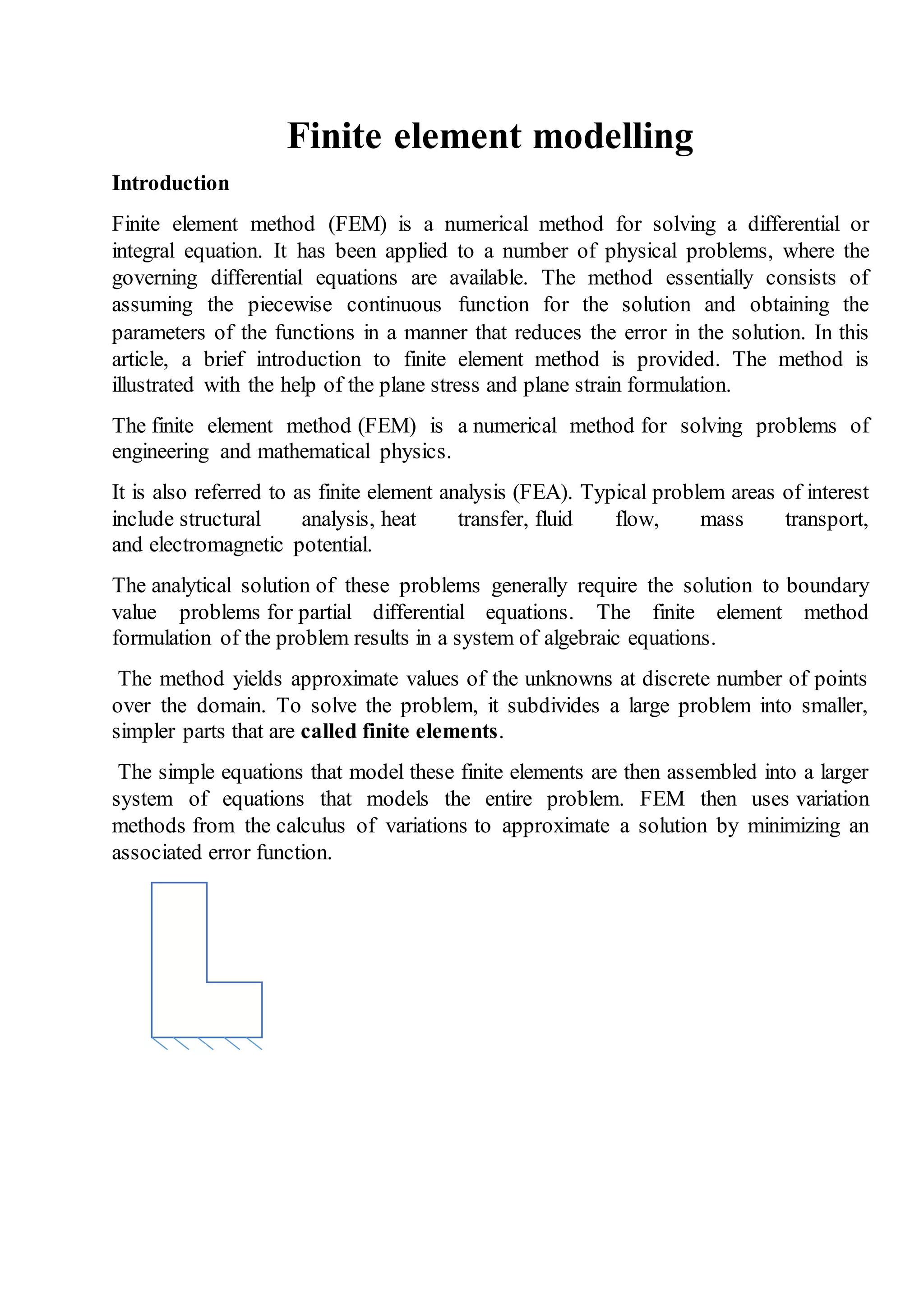
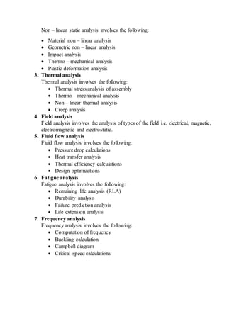
Finite element modelling
Introduction
Finite element method (FEM) is a numerical method for solving a differential or
integral equation. It has been applied to a number of physical problems, where the
governing differential equations are available. The method essentially consists of
assuming the piecewise continuous function for the solution and obtaining the
parameters of the functions in a manner that reduces the error in the solution. In this
article, a brief introduction to finite element method is provided. The method is
illustrated with the help of the plane stress and plane strain formulation.
The finite element method (FEM) is a numerical method for solving problems of
engineering and mathematical physics.
It is also referred to as finite element analysis (FEA). Typical problem areas of interest
include structural analysis, heat transfer, fluid flow, mass transport,
and electromagnetic potential.
The analytical solution of these problems generally require the solution to boundary
value problems for partial differential equations. The finite element method
formulation of the problem results in a system of algebraic equations.
The method yields approximate values of the unknowns at discrete number of points
over the domain. To solve the problem, it subdivides a large problem into smaller,
simpler parts that are called finite elements.
The simple equations that model these finite elements are then assembled into a larger
system of equations that models the entire problem. FEM then uses variation
methods from the calculus of variations to approximate a solution by minimizing an
associated error function.
Objectives of FEM
1. Understand the fundamental ideas of the FEM ·
2. Know the behaviour and usage of each type of elements covered in this course ·
3. Be able to prepare a suitable FE model for structural mechanical analysis
problems ·
4. Can interpret and evaluate the quality of the results (know the physics of the
problems).
5. Be aware of the limitations of the FEM (don't misuse the FEM - a numerical
tool).
Types of FEA (finite element analysis)
Finite element analysis is classified into the following types:
1. Structural analysis
2. Linear & non – linear analysis
3. Thermal analysis
4. Field analysis
5. Fluid flow analysis
6. Fatigue analysis
7. Frequency analysis
1. Structure analysis (dynamic analysis)
Structure analysis involves the following calculations
 Frequency response analysis
 Seismic analysis
 Harmonic analysis
 Shockcalculations
 Vibration calculations
2. Linear & non – linear analysis
Linear static analysis involves the following:
 Factorof safety calculations
 Deflections calculations
 Stiffness calculations
 Part & assembly stress analysis
Non – linear static analysis involves the following:
 Material non – linear analysis
 Geometric non – linear analysis
 Impact analysis
 Thermo – mechanical analysis
 Plastic deformation analysis
3. Thermal analysis
Thermal analysis involves the following:
 Thermal stress analysis of assembly
 Thermo – mechanical analysis
 Non – linear thermal analysis
 Creep analysis
4. Field analysis
Field analysis involves the analysis of types of the field i.e. electrical, magnetic,
electromagnetic and electrostatic.
5. Fluid flow analysis
Fluid flow analysis involves the following:
 Pressure drop calculations
 Heat transfer analysis
 Thermal efficiency calculations
 Design optimizations
6. Fatigue analysis
Fatigue analysis involves the following:
 Remaining life analysis (RLA)
 Durability analysis
 Failure prediction analysis
 Life extension analysis
7. Frequency analysis
Frequency analysis involves the following:
 Computation of frequency
 Buckling calculation
 Campbell diagram
 Critical speed calculations
Degree of freedom
The deformation of structure is referred as the displacement of node. These
displacements are known as degree of freedom. DOF is defined as the structure which
have translation (x, y, z axis) as well as rotational (x, y, z direction) motion.
Cantilever beam
The node of element has three D.O.F
Y vi ui
X vj uj
Again a two-dimensional case with a single field variable φ(x, y). The triangular
element described is said to have 3 degrees of freedom, as three nodal values of the
field variable are required to describe the field variable everywhere in the element
(scalar).
In general, the number of degrees of freedom associated with a finite element is equal
to the product of the number of nodes and the number of values of the field variable
(and possibly its derivatives) that must be computed at each node.
φ(x, y) = N1(x, y) φ1 + N2(x, y) φ2 + N3(x, y) φ3
Flounce coefficient
Three conditions are required to solve any structure problem:
1. Equilibrium of force
2. Compability of deformation
3. Material behaviour
1
3 2
The system equation for FEM is ;
[k] {u} = {f}
Where, [k] = stiffness matrix
{u} = displacement vector
{f} = free vector
 A stiffness matrix is collection of the term is called influence coefficient. An
influence coefficient relating to force at a point to the displacement is called
stiffness influence coefficient.
𝑭 = 𝒌 𝟏𝟏 𝒖 𝟏𝟏 + 𝒌 𝟏𝟐 𝒖 𝟏𝟐 + 𝒌 𝟏𝟑 𝒖 𝟏𝟑 + ………………… . . 𝒌 𝟏𝒏 𝒖 𝟏𝒏
(𝒊 = 𝟏 𝒕𝒐 𝒏)
Element and stiffness equation
Finite element model can be constructed out of the spring element, beam, plate, shell,
pipe, and the solid. Commonly used element is spring element. A linear elastic spring
is a mechanical device capable of supporting axial loading only, and the elongation or
contraction of the spring is directly proportional to the applied axial load. The constant
of proportionality between deformation and load is referred to as the spring constant,
spring rate, or spring stiffness k, and has units of force per unit length. As an elastic
spring supports axial loading only, we select an element coordinate system (also
known as a local coordinate system) as an x axis oriented along the length of the
spring, as shown.
Spring element:. A spring element is shown in the fig. below;
Fi Vi Vj Fj
Let i and j be nodes of element and Fi, Fj be the force on ith and jth node.
Influence coefficient = 𝑘𝑖𝑗 = −𝑘𝑗𝑖 = +𝑘
In matrix form,
[
𝑘 −𝑘
−𝑘 𝑘
][
𝑢𝑖
𝑢𝑗
] = [
𝑓𝑖
𝑓𝑗
]
Spring elements can be assembled on the basis of superposition principle:
[
𝑢1 𝑢2 𝑢3
𝑘 −𝑘 0
−𝑘 𝑘 0
] for element 2, stiffness matrix is; [
𝑢1 𝑢2 𝑢3
0 +𝑘 −𝑘
0 −𝑘 𝑘
]
Adding element 1 & 2, then resultant matrix is;
[
𝑘 −𝑘 0
−𝑘 𝑘 + 𝑘 −𝑘
0 −𝑘 𝑘
]
The equation of spring system becomes;
[
𝑘 −𝑘 0
−𝑘 𝑘 + 𝑘 −𝑘
0 −𝑘 𝑘
] [
𝑢1
𝑢2
𝑢3
] = [
𝑓1
𝑓2
𝑓3
]
But 𝑓3 = 𝑓 & 𝑢1 = 0
[
𝑘22 𝑘23
𝑘32 𝑘33
][
𝑢2
𝑢3
] = [
0
𝑓
]
[𝑘12 𝑘13][
𝑢2
𝑢3
] = 𝑓1
Equation 1 is known as the stiffness equation for the spring element taken above.
Procedure for finite element analysis
FEA can be performed into following steps:
1. Discretization: In this step the entire body to be analysed is divided into
smaller or finite elements. The finite elements are categorized by:
a. Family
b.Order
c.Tropology
Family of element refers to the characteristics of geometry and displacement.
Some common families are beam, thin shells & solid.
Node
Element
The order of the elements refers to the order of equations as linear, parabolic or cubic.
Element topology refers to the general shape of the element, such as triangular or
quadrilateral.
rec
2. Choosing the solution approximation: It refers to the finding values of field
variation at nodes of elements by using polynomial expressions, differentiation
and integration.
3. Forming the element matrix equation: The analysis of a single matrix is done
by applying equations of equilibrium to that element. These equations can be
expressed in the form of a matrix called element – matrix.
4. Assembling the matrix: The matrix of element is assembled to form the global
stiffness matrix. The boundary conditions can be used to reduce the size
stiffness matrix. It contains all the information of matrix.
5. Finding the unknown field variables: The unknown field variables from
global stiffness matrix can be calculated by using gauss elimination method.
6. Interpreting the results: Once the value of field variable is obtained, the
conclusions are drawn, modified and incorporated into original design.

Finite element modelling

  • 1.
    Finite element modelling Introduction Finiteelement method (FEM) is a numerical method for solving a differential or integral equation. It has been applied to a number of physical problems, where the governing differential equations are available. The method essentially consists of assuming the piecewise continuous function for the solution and obtaining the parameters of the functions in a manner that reduces the error in the solution. In this article, a brief introduction to finite element method is provided. The method is illustrated with the help of the plane stress and plane strain formulation. The finite element method (FEM) is a numerical method for solving problems of engineering and mathematical physics. It is also referred to as finite element analysis (FEA). Typical problem areas of interest include structural analysis, heat transfer, fluid flow, mass transport, and electromagnetic potential. The analytical solution of these problems generally require the solution to boundary value problems for partial differential equations. The finite element method formulation of the problem results in a system of algebraic equations. The method yields approximate values of the unknowns at discrete number of points over the domain. To solve the problem, it subdivides a large problem into smaller, simpler parts that are called finite elements. The simple equations that model these finite elements are then assembled into a larger system of equations that models the entire problem. FEM then uses variation methods from the calculus of variations to approximate a solution by minimizing an associated error function.
  • 2.
    Objectives of FEM 1.Understand the fundamental ideas of the FEM · 2. Know the behaviour and usage of each type of elements covered in this course · 3. Be able to prepare a suitable FE model for structural mechanical analysis problems · 4. Can interpret and evaluate the quality of the results (know the physics of the problems). 5. Be aware of the limitations of the FEM (don't misuse the FEM - a numerical tool). Types of FEA (finite element analysis) Finite element analysis is classified into the following types: 1. Structural analysis 2. Linear & non – linear analysis 3. Thermal analysis 4. Field analysis 5. Fluid flow analysis 6. Fatigue analysis 7. Frequency analysis 1. Structure analysis (dynamic analysis) Structure analysis involves the following calculations  Frequency response analysis  Seismic analysis  Harmonic analysis  Shockcalculations  Vibration calculations 2. Linear & non – linear analysis Linear static analysis involves the following:  Factorof safety calculations  Deflections calculations  Stiffness calculations  Part & assembly stress analysis
  • 3.
    Non – linearstatic analysis involves the following:  Material non – linear analysis  Geometric non – linear analysis  Impact analysis  Thermo – mechanical analysis  Plastic deformation analysis 3. Thermal analysis Thermal analysis involves the following:  Thermal stress analysis of assembly  Thermo – mechanical analysis  Non – linear thermal analysis  Creep analysis 4. Field analysis Field analysis involves the analysis of types of the field i.e. electrical, magnetic, electromagnetic and electrostatic. 5. Fluid flow analysis Fluid flow analysis involves the following:  Pressure drop calculations  Heat transfer analysis  Thermal efficiency calculations  Design optimizations 6. Fatigue analysis Fatigue analysis involves the following:  Remaining life analysis (RLA)  Durability analysis  Failure prediction analysis  Life extension analysis 7. Frequency analysis Frequency analysis involves the following:  Computation of frequency  Buckling calculation  Campbell diagram  Critical speed calculations
  • 4.
    Degree of freedom Thedeformation of structure is referred as the displacement of node. These displacements are known as degree of freedom. DOF is defined as the structure which have translation (x, y, z axis) as well as rotational (x, y, z direction) motion. Cantilever beam The node of element has three D.O.F Y vi ui X vj uj Again a two-dimensional case with a single field variable φ(x, y). The triangular element described is said to have 3 degrees of freedom, as three nodal values of the field variable are required to describe the field variable everywhere in the element (scalar). In general, the number of degrees of freedom associated with a finite element is equal to the product of the number of nodes and the number of values of the field variable (and possibly its derivatives) that must be computed at each node. φ(x, y) = N1(x, y) φ1 + N2(x, y) φ2 + N3(x, y) φ3 Flounce coefficient Three conditions are required to solve any structure problem: 1. Equilibrium of force 2. Compability of deformation 3. Material behaviour 1 3 2
  • 5.
    The system equationfor FEM is ; [k] {u} = {f} Where, [k] = stiffness matrix {u} = displacement vector {f} = free vector  A stiffness matrix is collection of the term is called influence coefficient. An influence coefficient relating to force at a point to the displacement is called stiffness influence coefficient. 𝑭 = 𝒌 𝟏𝟏 𝒖 𝟏𝟏 + 𝒌 𝟏𝟐 𝒖 𝟏𝟐 + 𝒌 𝟏𝟑 𝒖 𝟏𝟑 + ………………… . . 𝒌 𝟏𝒏 𝒖 𝟏𝒏 (𝒊 = 𝟏 𝒕𝒐 𝒏) Element and stiffness equation Finite element model can be constructed out of the spring element, beam, plate, shell, pipe, and the solid. Commonly used element is spring element. A linear elastic spring is a mechanical device capable of supporting axial loading only, and the elongation or contraction of the spring is directly proportional to the applied axial load. The constant of proportionality between deformation and load is referred to as the spring constant, spring rate, or spring stiffness k, and has units of force per unit length. As an elastic spring supports axial loading only, we select an element coordinate system (also known as a local coordinate system) as an x axis oriented along the length of the spring, as shown. Spring element:. A spring element is shown in the fig. below; Fi Vi Vj Fj Let i and j be nodes of element and Fi, Fj be the force on ith and jth node. Influence coefficient = 𝑘𝑖𝑗 = −𝑘𝑗𝑖 = +𝑘 In matrix form, [ 𝑘 −𝑘 −𝑘 𝑘 ][ 𝑢𝑖 𝑢𝑗 ] = [ 𝑓𝑖 𝑓𝑗 ] Spring elements can be assembled on the basis of superposition principle: [ 𝑢1 𝑢2 𝑢3 𝑘 −𝑘 0 −𝑘 𝑘 0 ] for element 2, stiffness matrix is; [ 𝑢1 𝑢2 𝑢3 0 +𝑘 −𝑘 0 −𝑘 𝑘 ]
  • 6.
    Adding element 1& 2, then resultant matrix is; [ 𝑘 −𝑘 0 −𝑘 𝑘 + 𝑘 −𝑘 0 −𝑘 𝑘 ] The equation of spring system becomes; [ 𝑘 −𝑘 0 −𝑘 𝑘 + 𝑘 −𝑘 0 −𝑘 𝑘 ] [ 𝑢1 𝑢2 𝑢3 ] = [ 𝑓1 𝑓2 𝑓3 ] But 𝑓3 = 𝑓 & 𝑢1 = 0 [ 𝑘22 𝑘23 𝑘32 𝑘33 ][ 𝑢2 𝑢3 ] = [ 0 𝑓 ] [𝑘12 𝑘13][ 𝑢2 𝑢3 ] = 𝑓1 Equation 1 is known as the stiffness equation for the spring element taken above. Procedure for finite element analysis FEA can be performed into following steps: 1. Discretization: In this step the entire body to be analysed is divided into smaller or finite elements. The finite elements are categorized by: a. Family b.Order c.Tropology Family of element refers to the characteristics of geometry and displacement. Some common families are beam, thin shells & solid. Node Element The order of the elements refers to the order of equations as linear, parabolic or cubic. Element topology refers to the general shape of the element, such as triangular or quadrilateral. rec
  • 7.
    2. Choosing thesolution approximation: It refers to the finding values of field variation at nodes of elements by using polynomial expressions, differentiation and integration. 3. Forming the element matrix equation: The analysis of a single matrix is done by applying equations of equilibrium to that element. These equations can be expressed in the form of a matrix called element – matrix. 4. Assembling the matrix: The matrix of element is assembled to form the global stiffness matrix. The boundary conditions can be used to reduce the size stiffness matrix. It contains all the information of matrix. 5. Finding the unknown field variables: The unknown field variables from global stiffness matrix can be calculated by using gauss elimination method. 6. Interpreting the results: Once the value of field variable is obtained, the conclusions are drawn, modified and incorporated into original design.