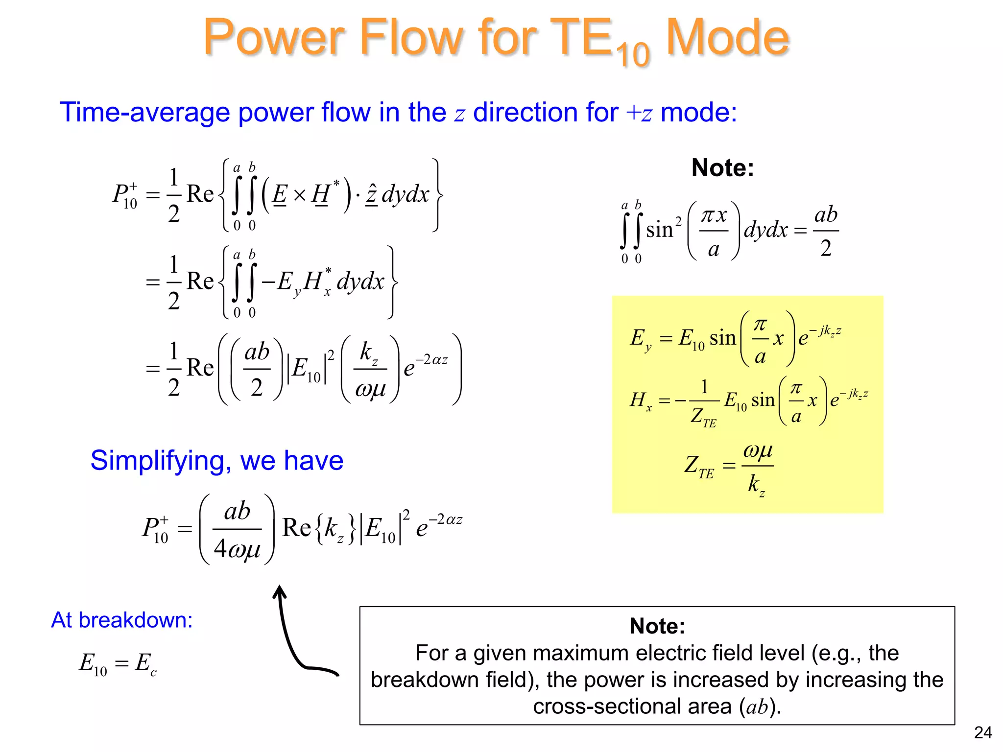
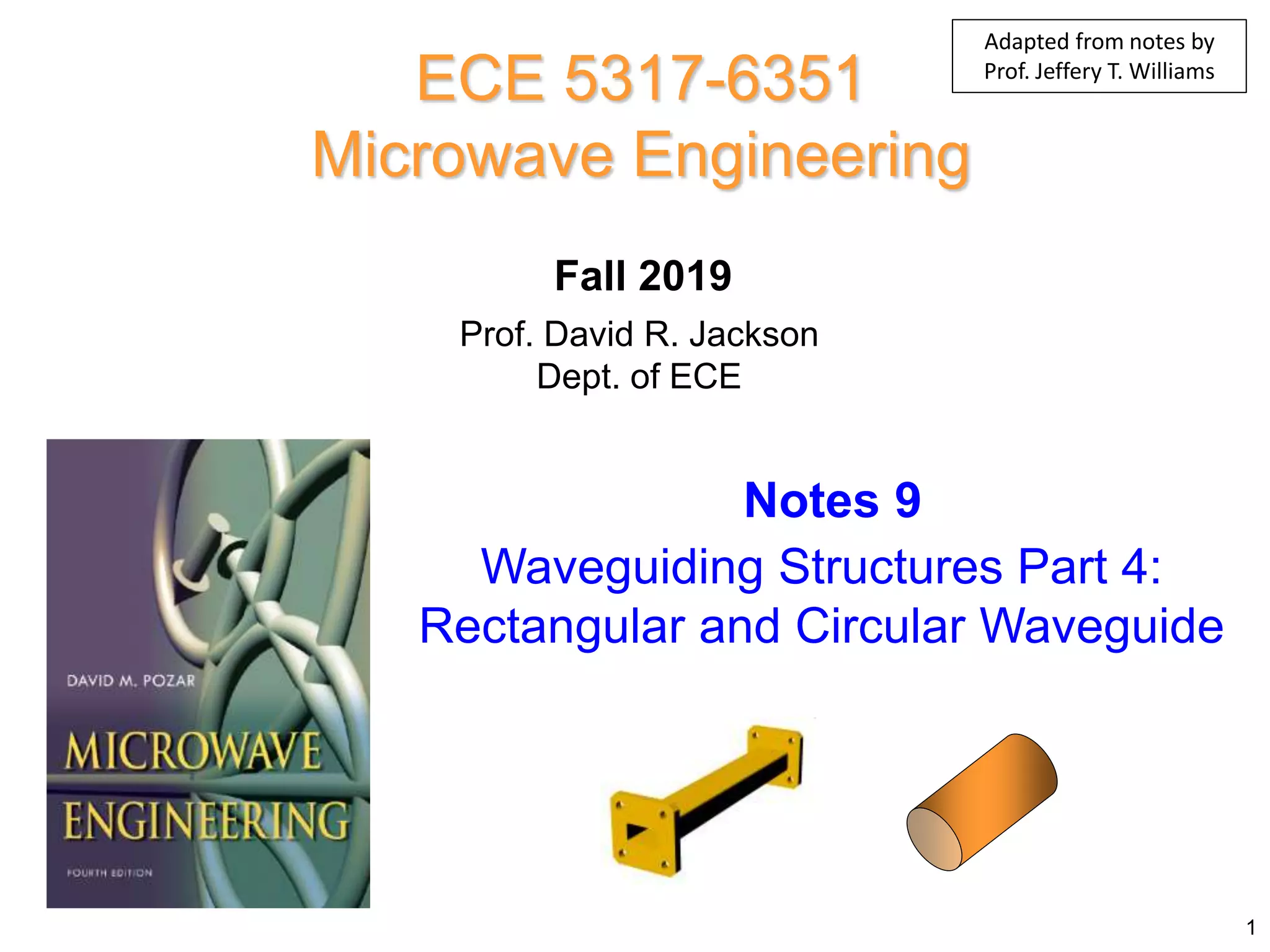
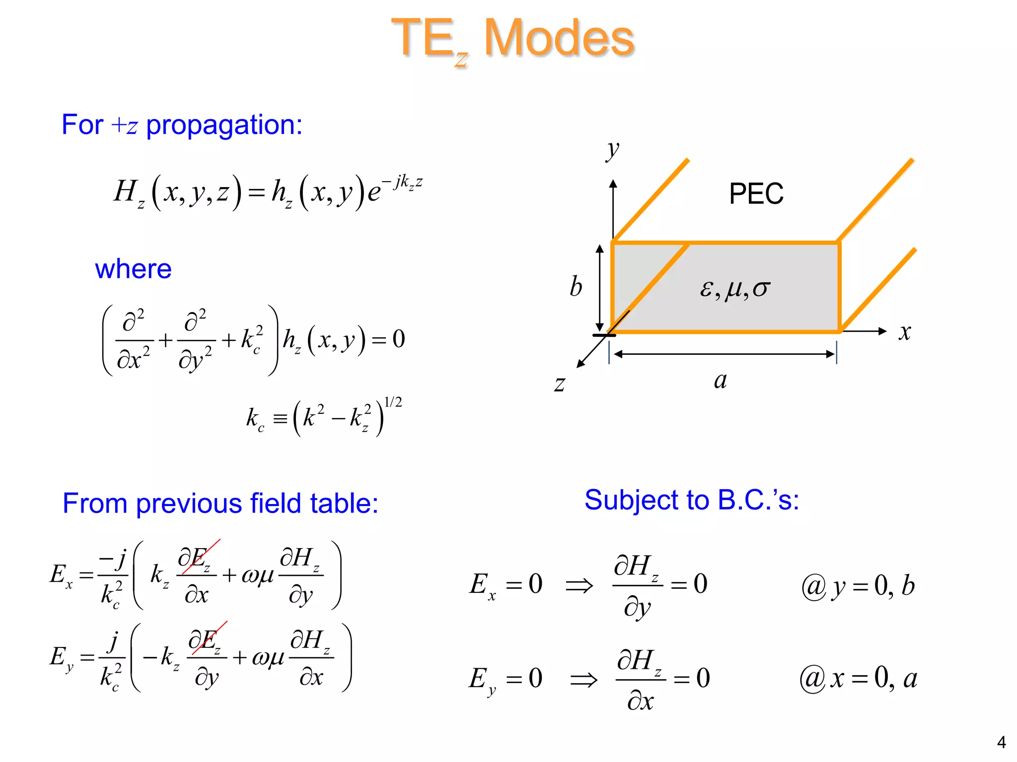
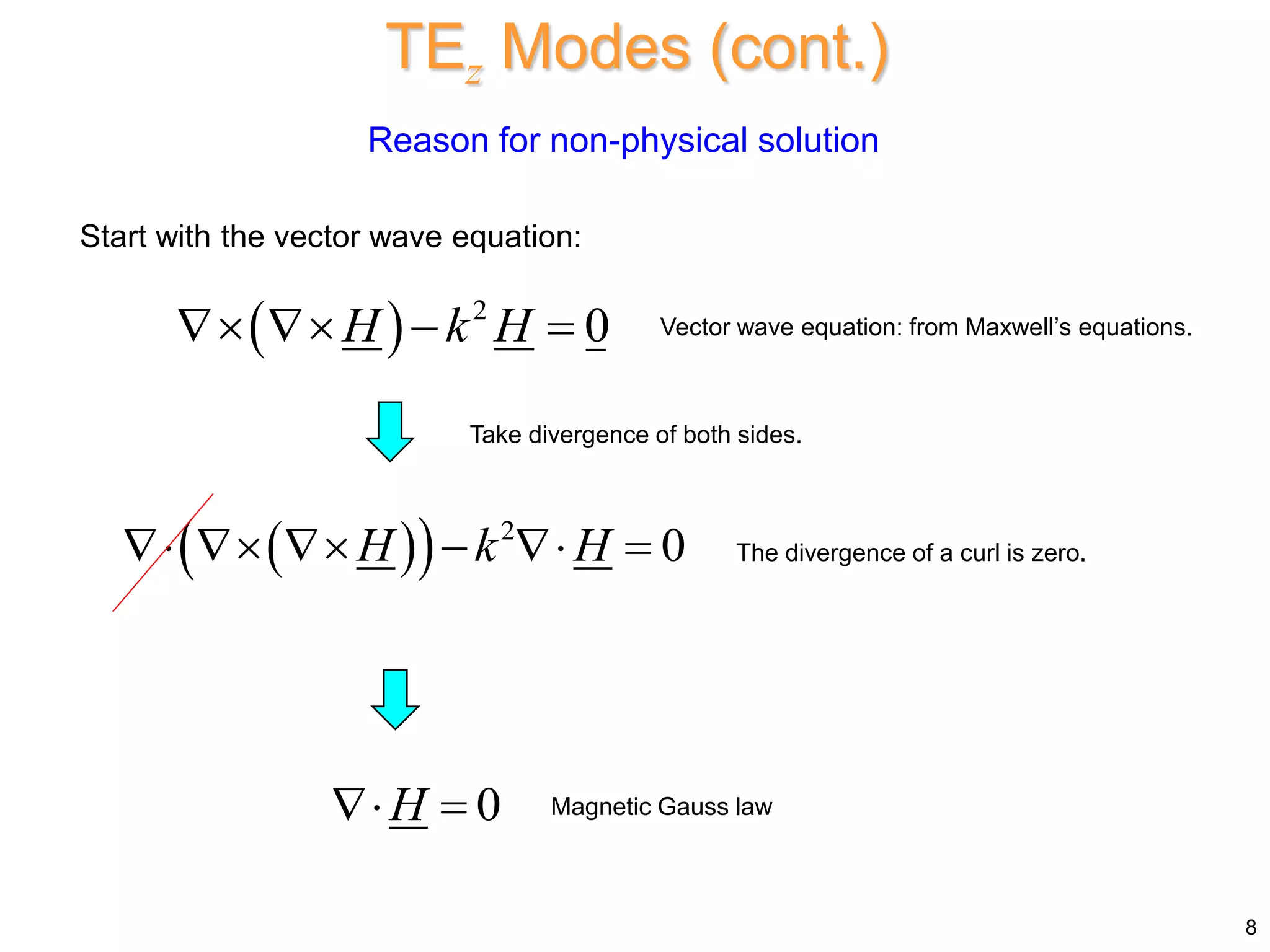
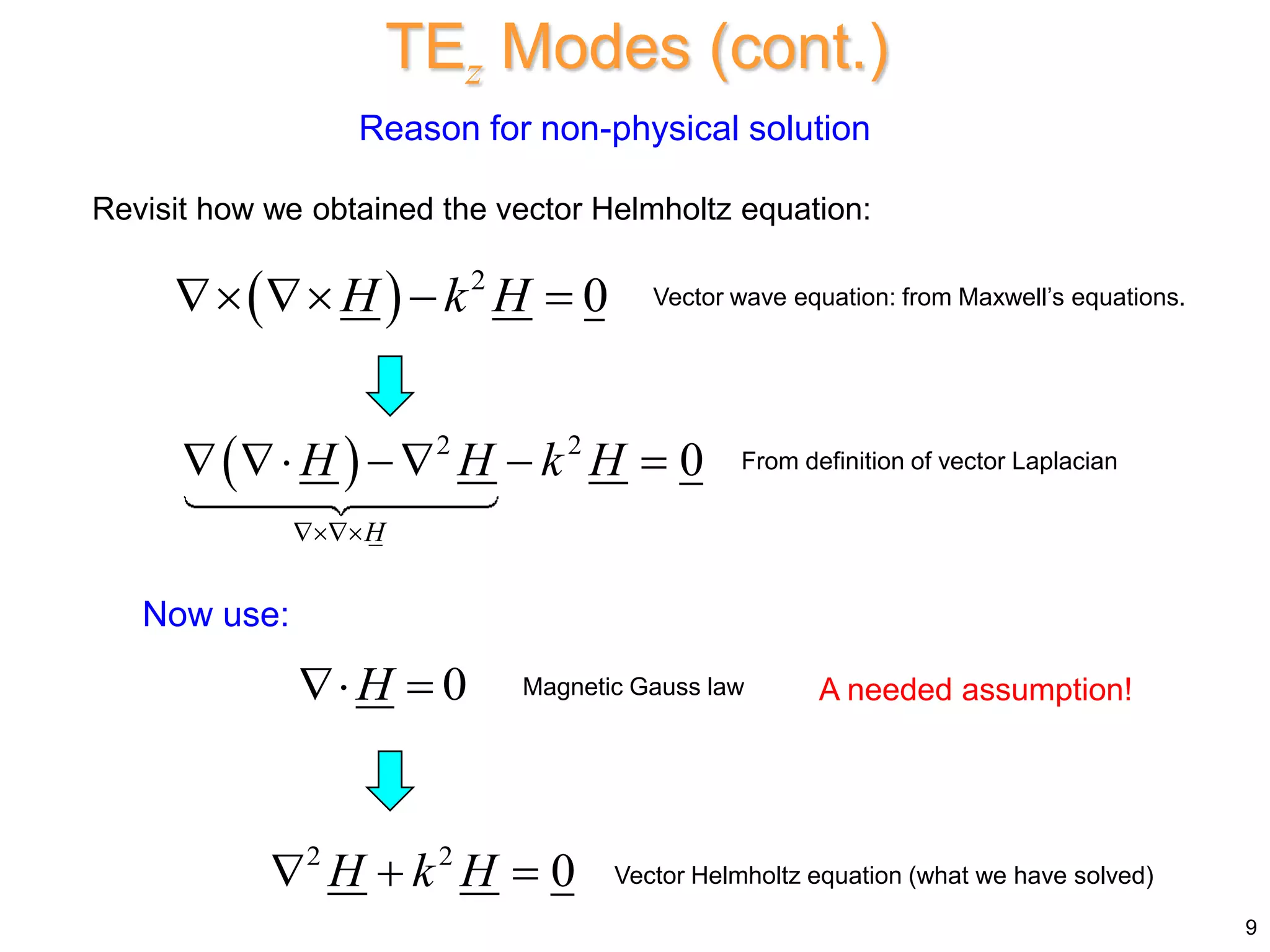
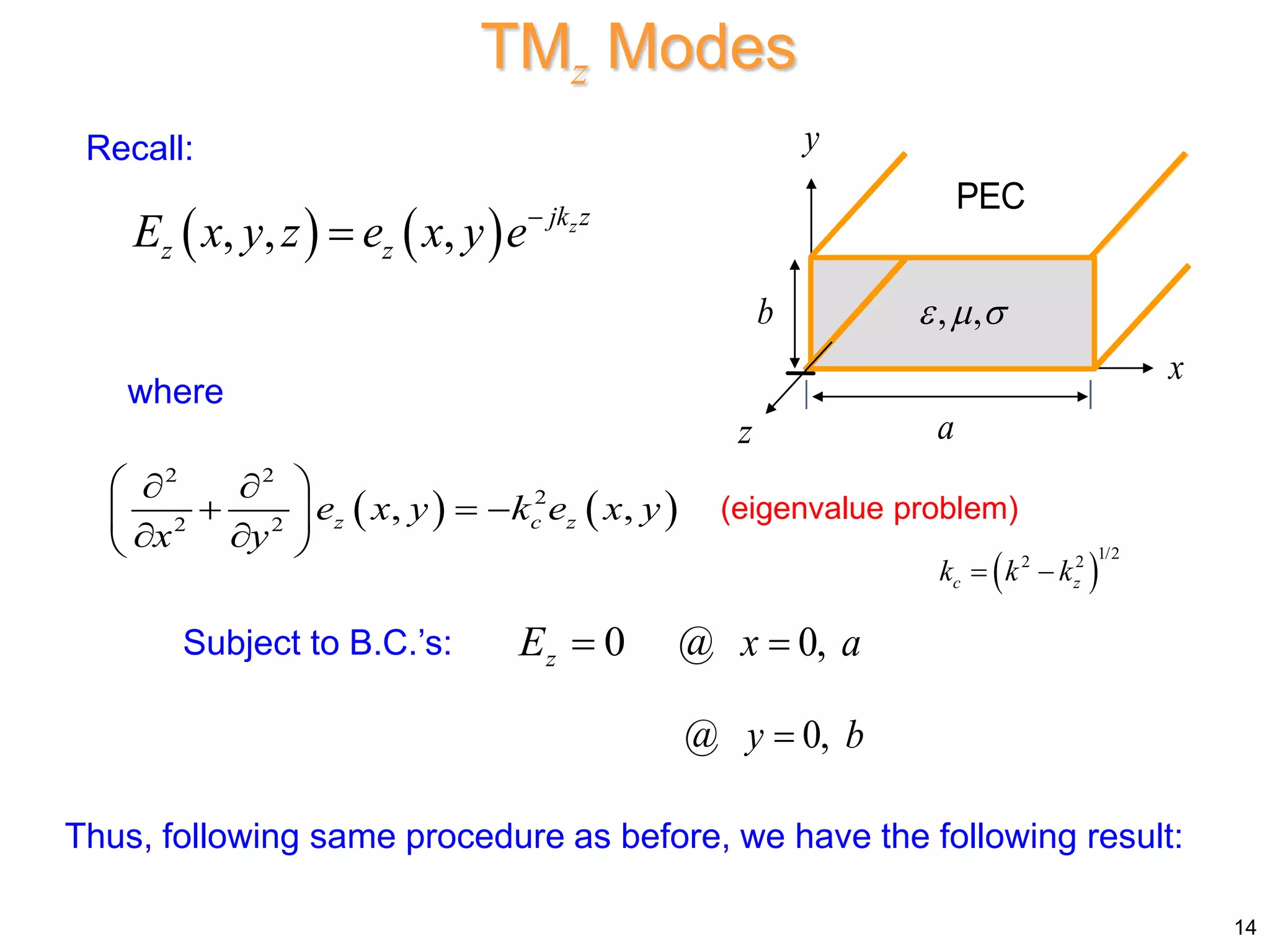
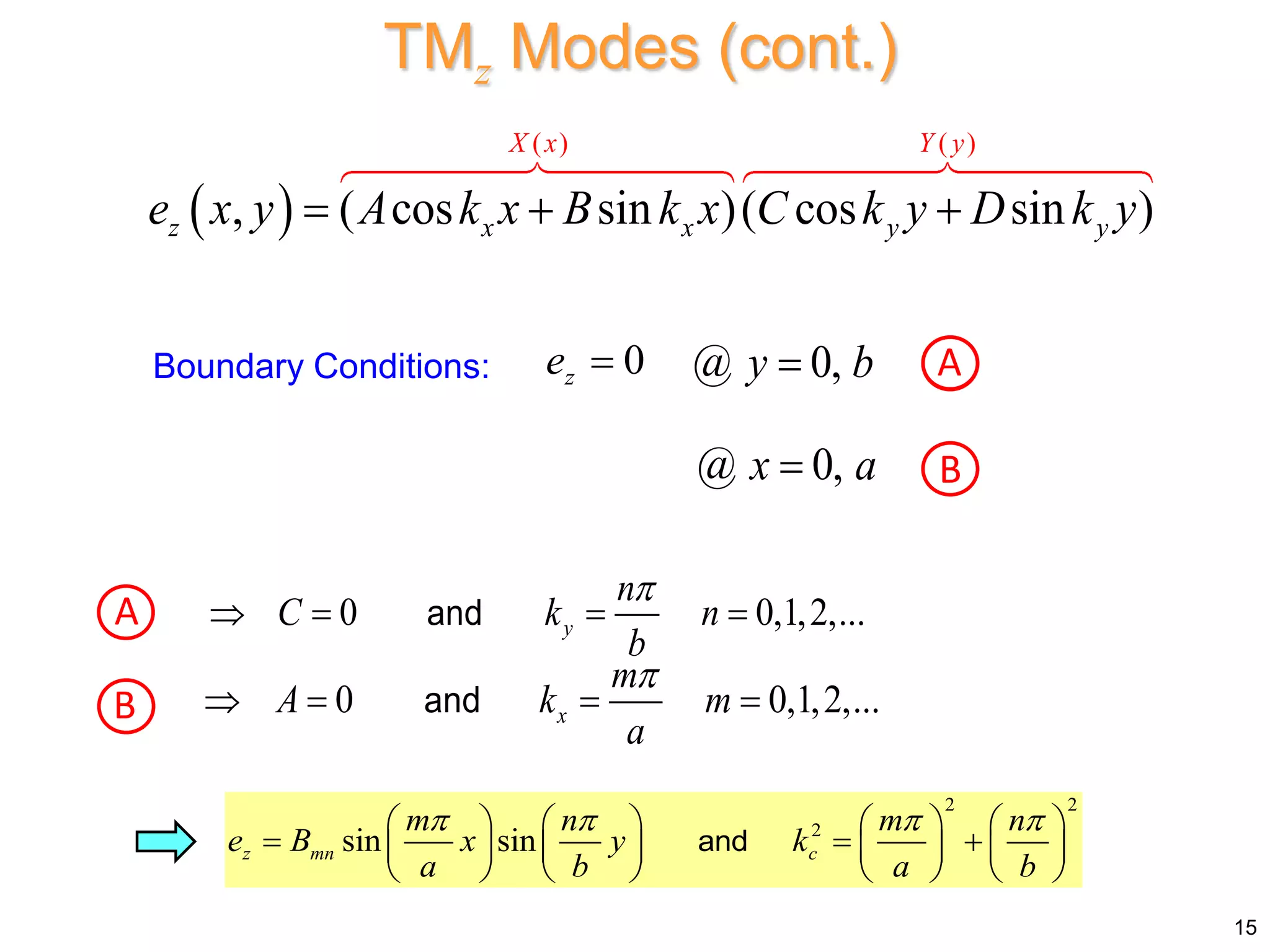
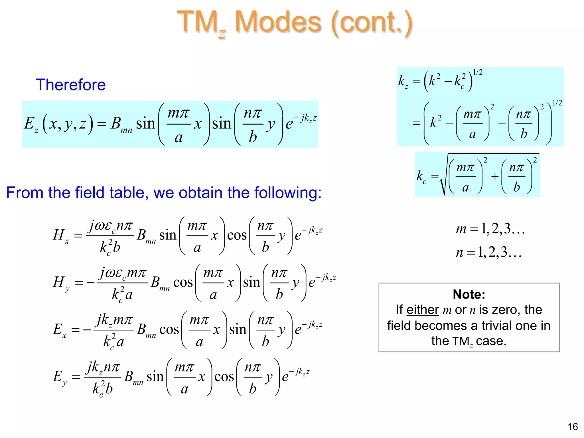
1) Rectangular waveguides are commonly used for high power and low-loss microwave and millimeter-wave applications. They guide waves through a rectangular cross-section pipe. 2) Waves can propagate through rectangular waveguides in transverse electric (TE) or transverse magnetic (TM) modes. The TE and TM modes are derived from solving Maxwell's equations subject to the boundary conditions of the waveguide walls. 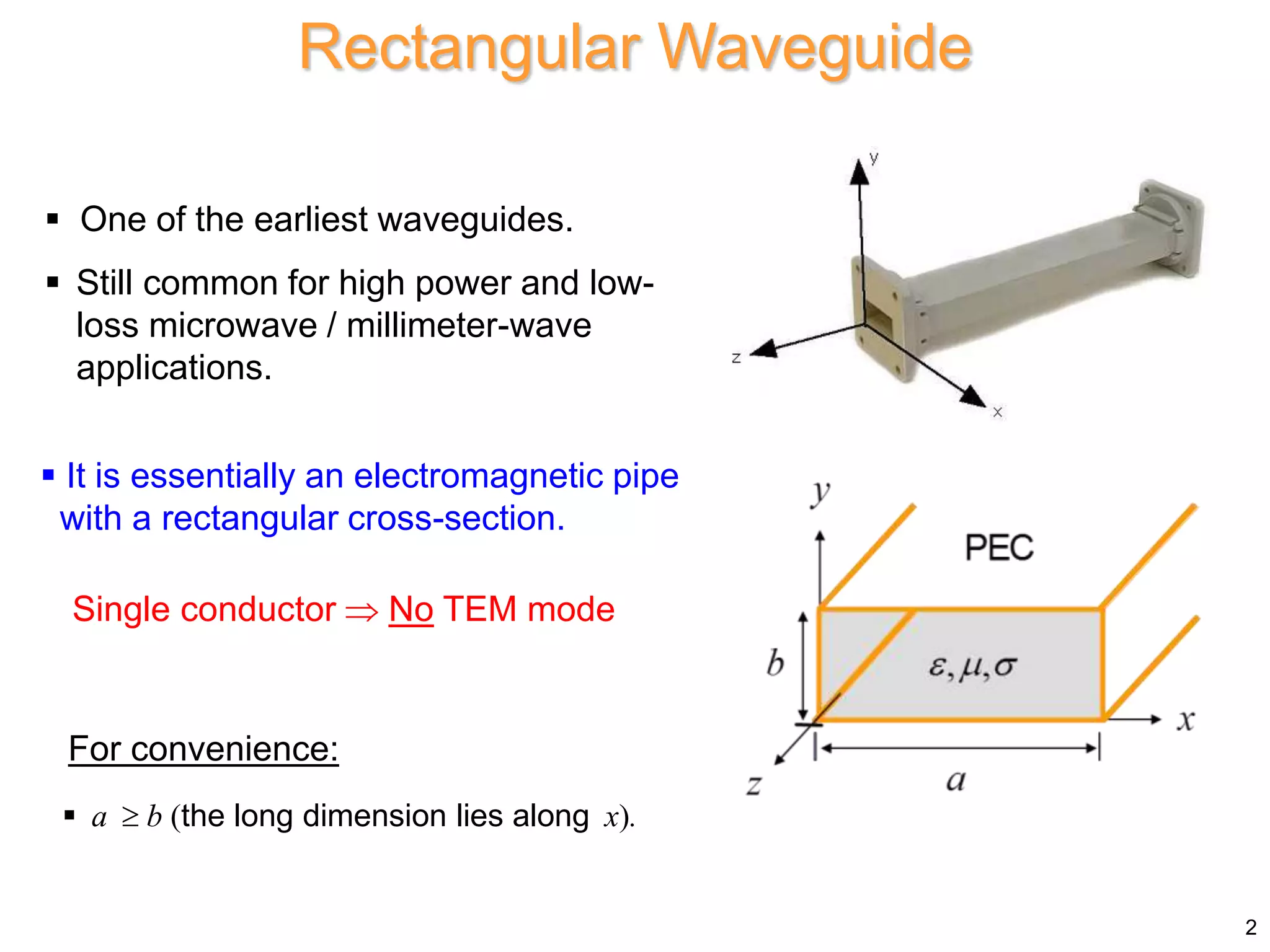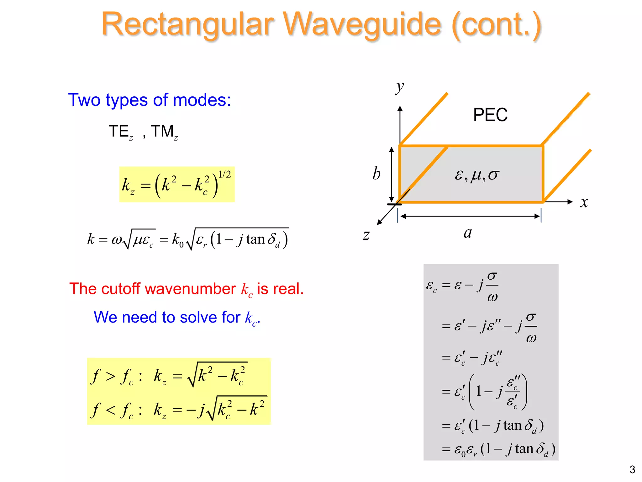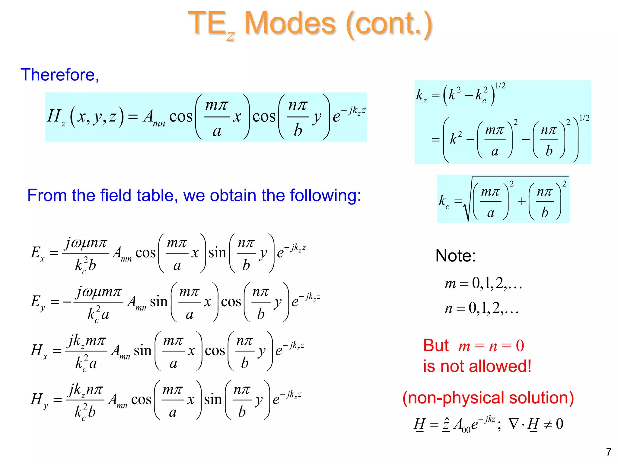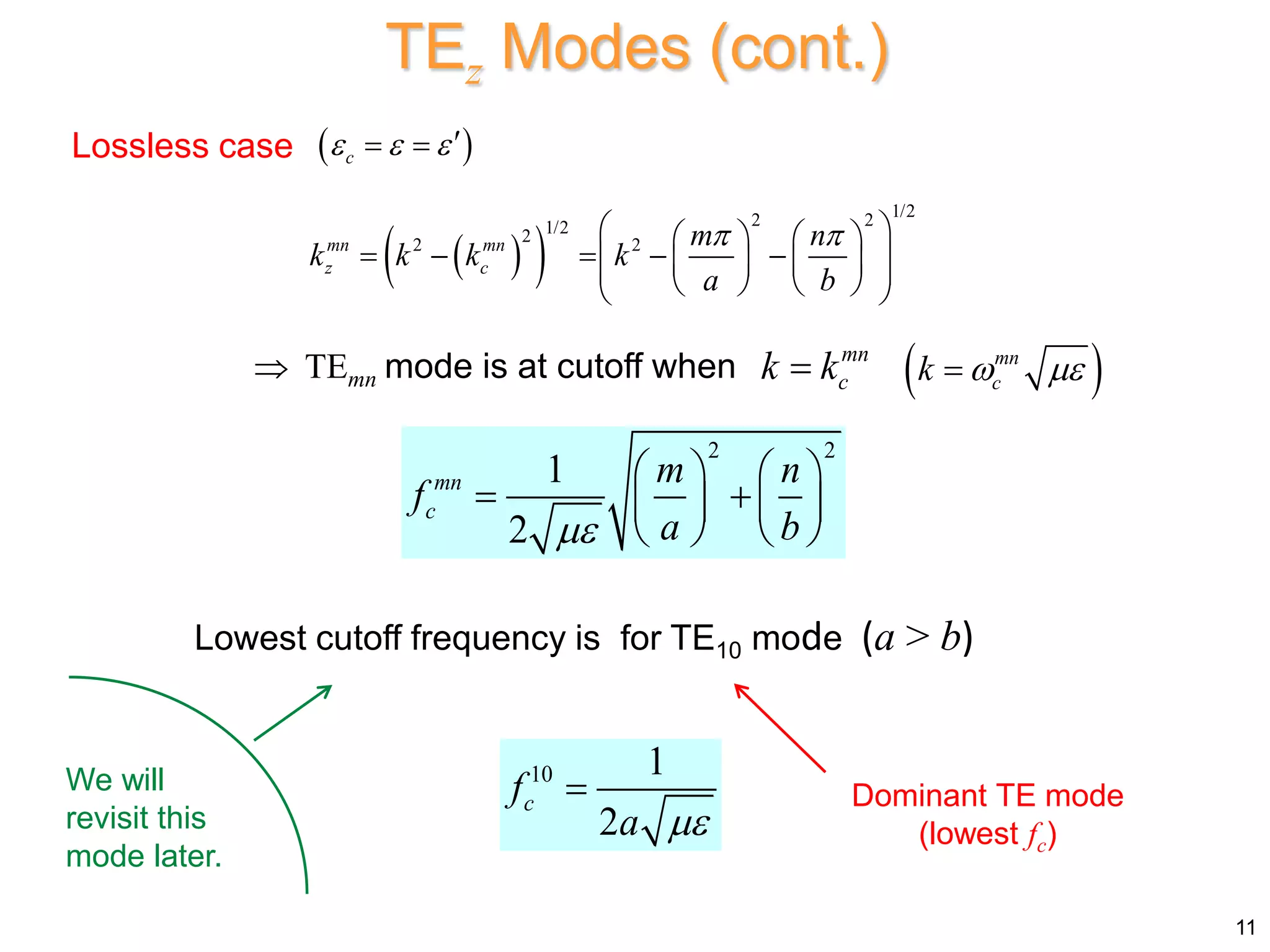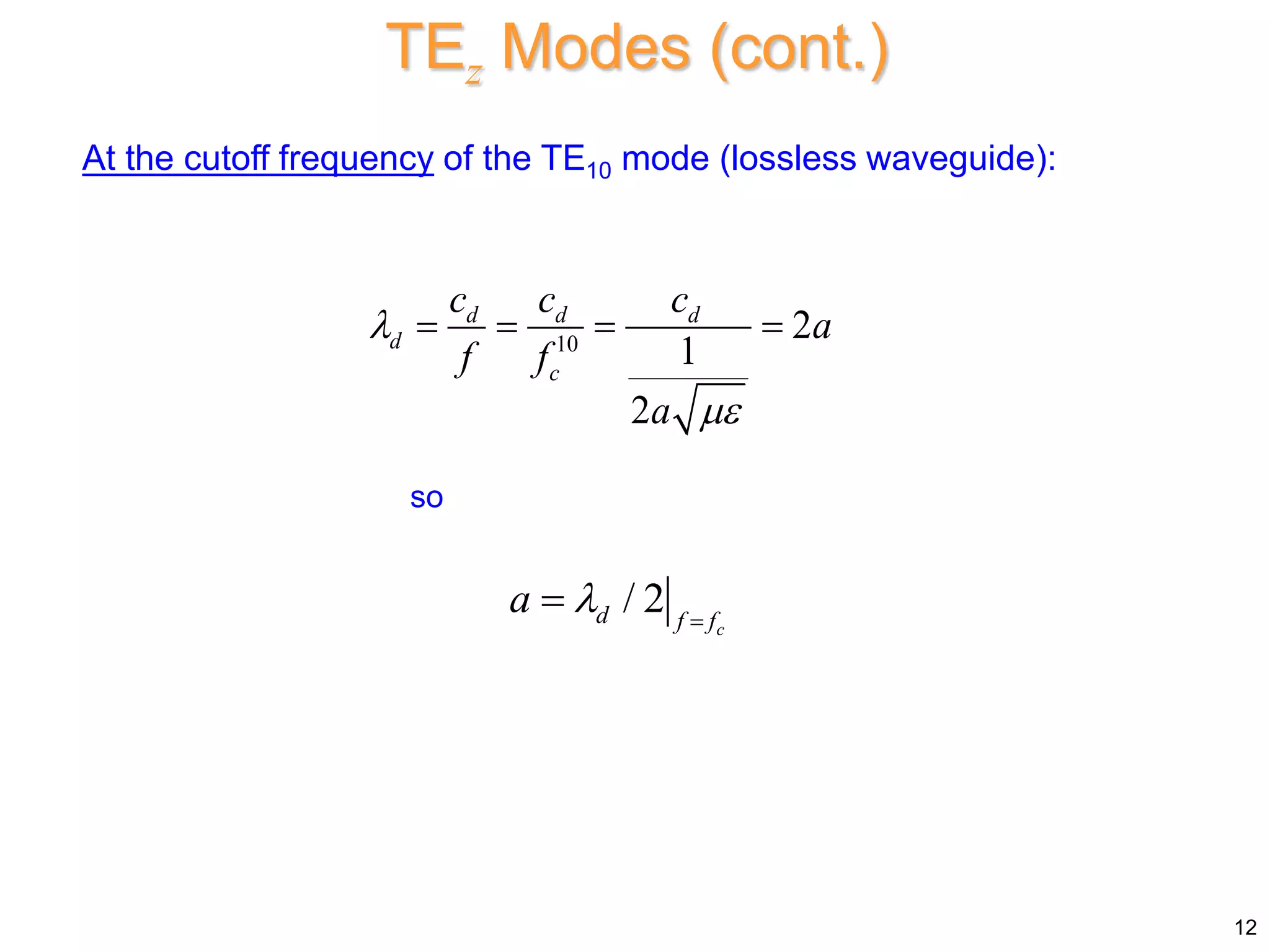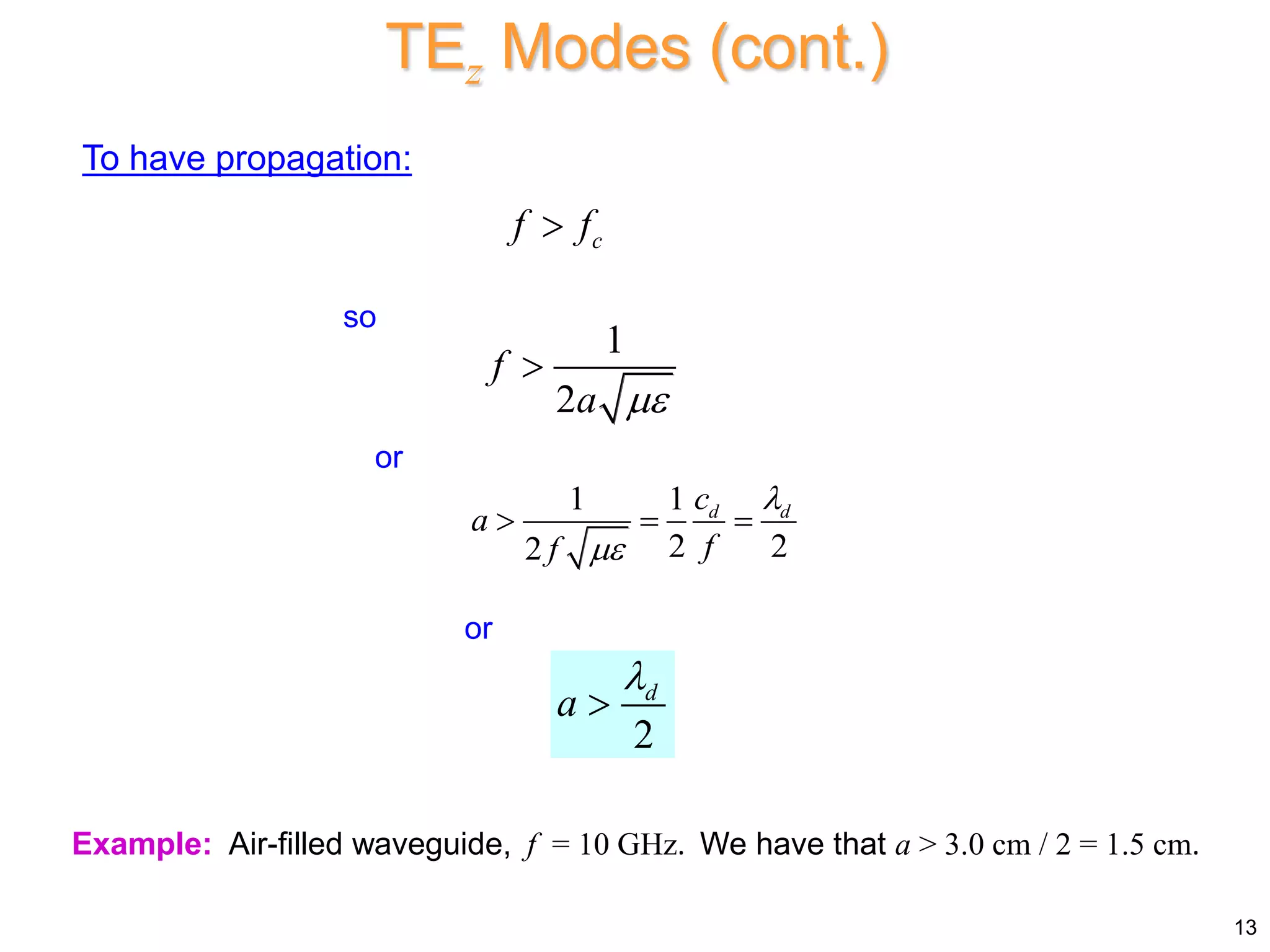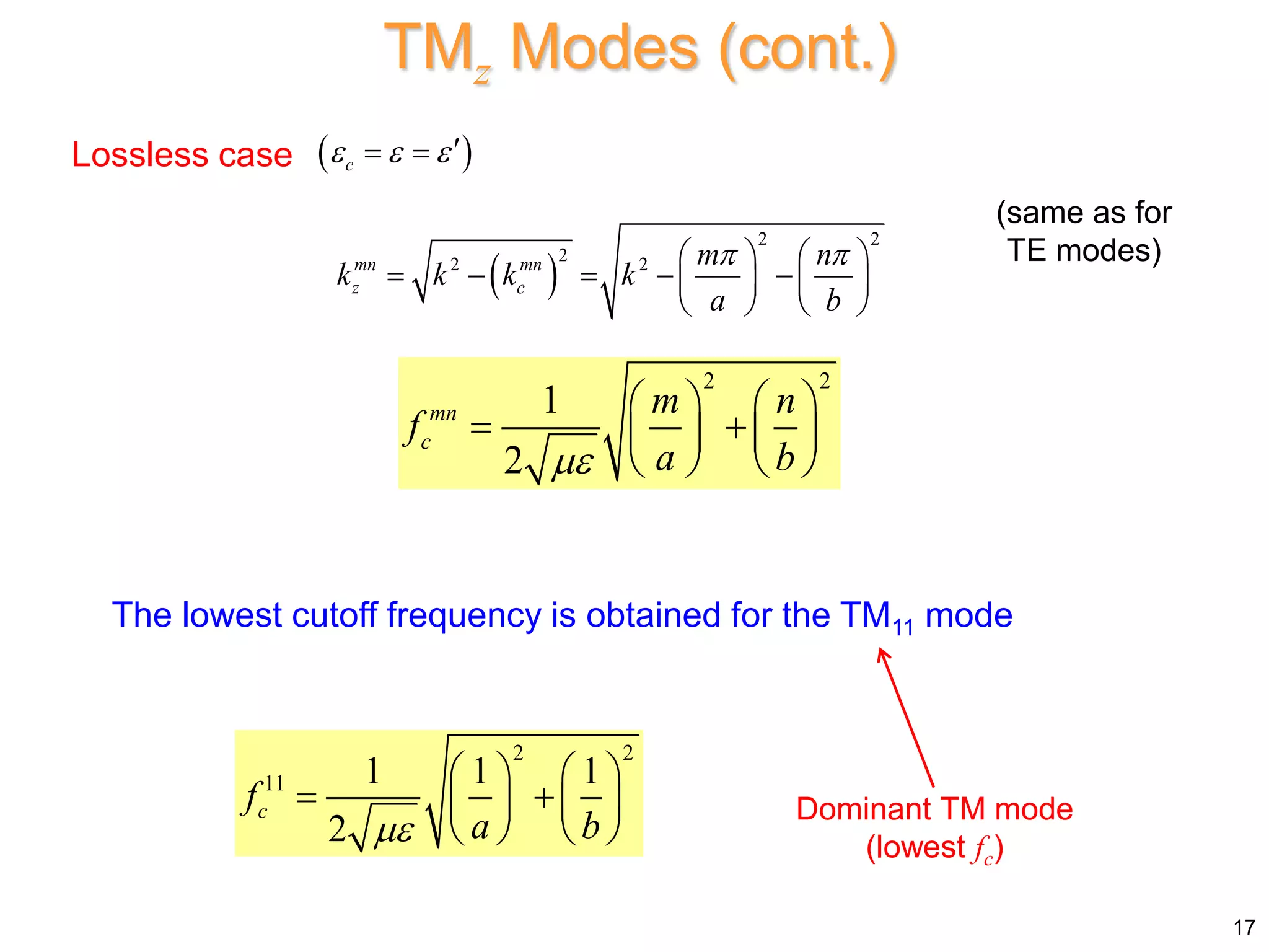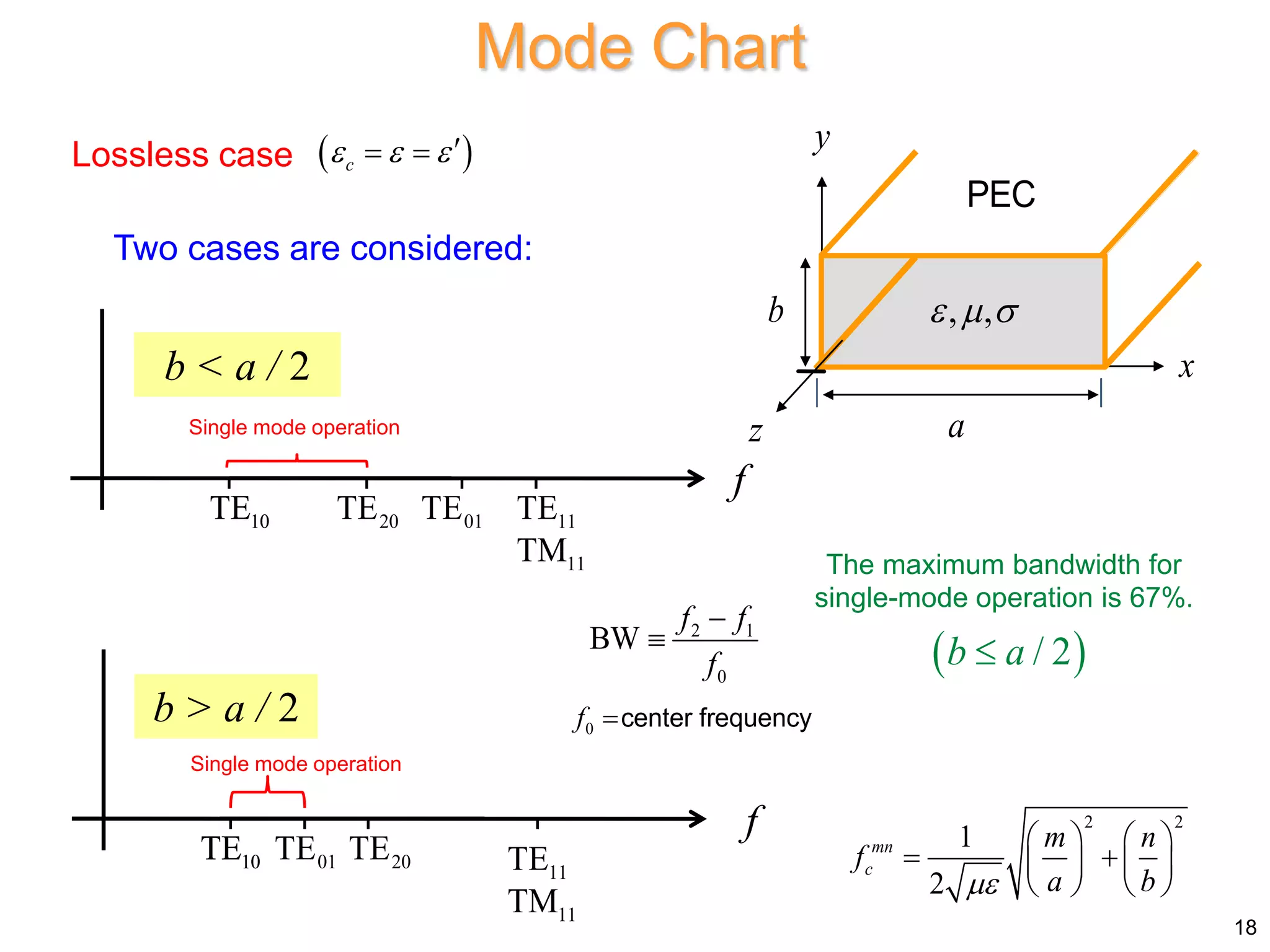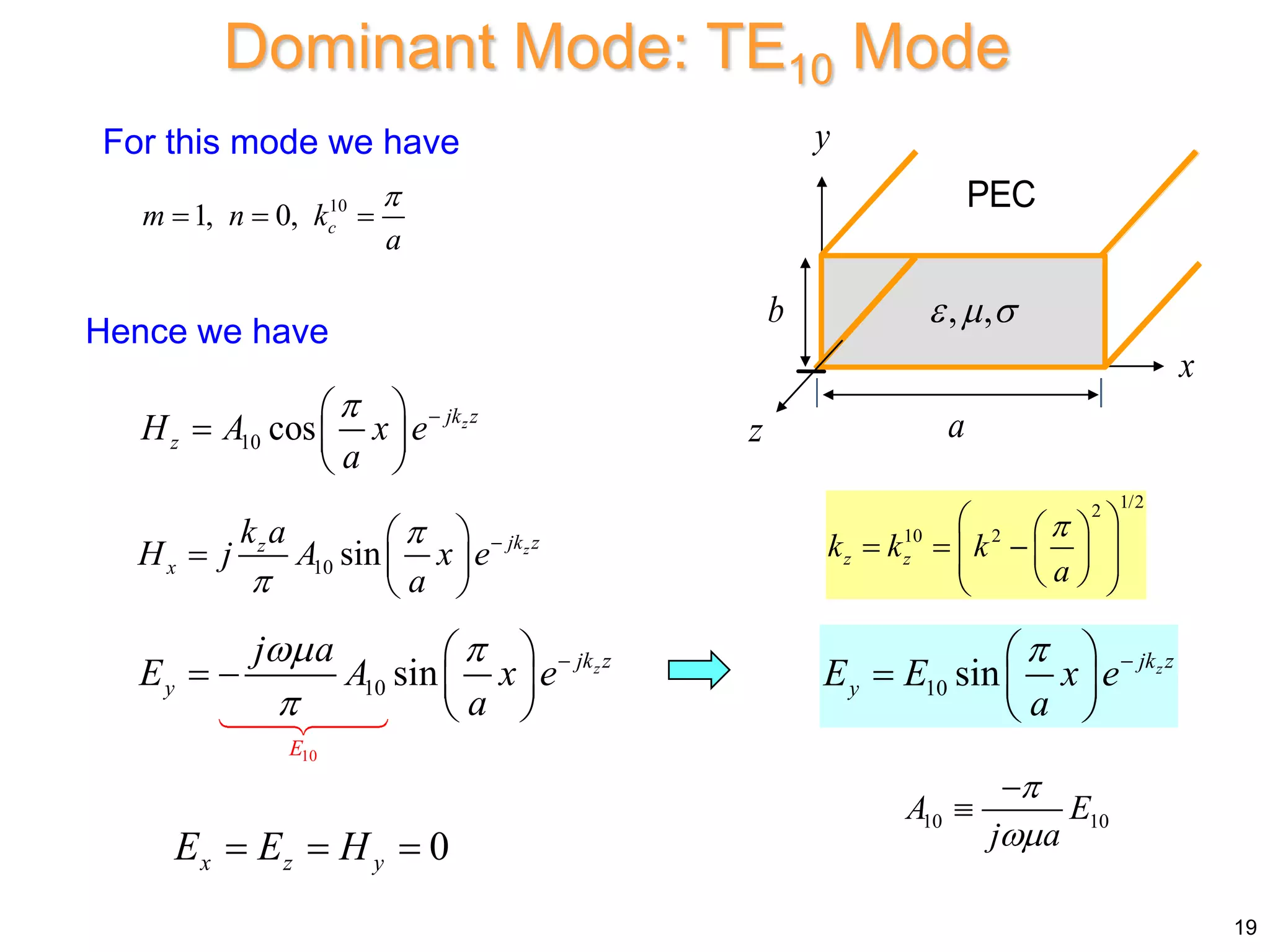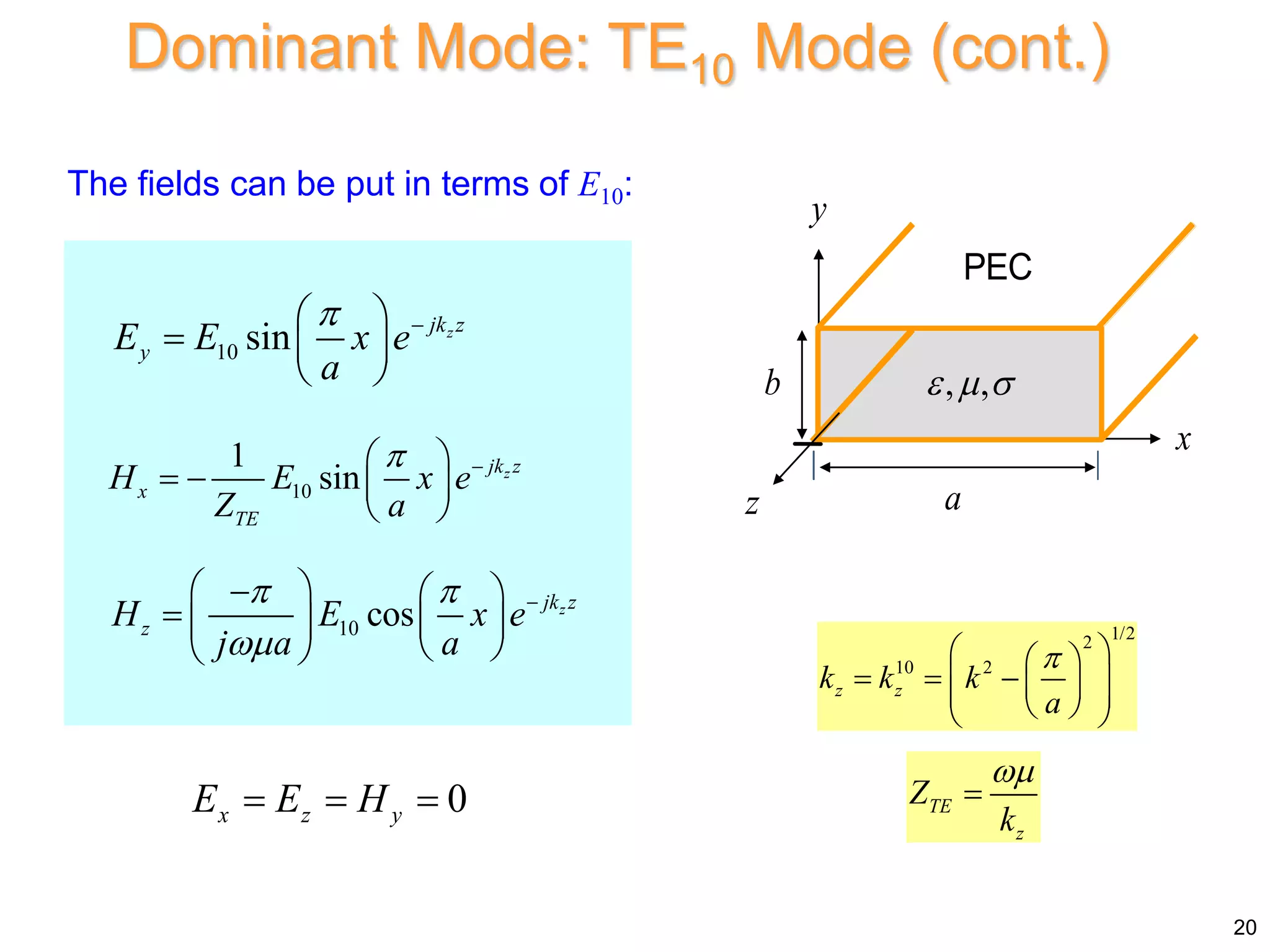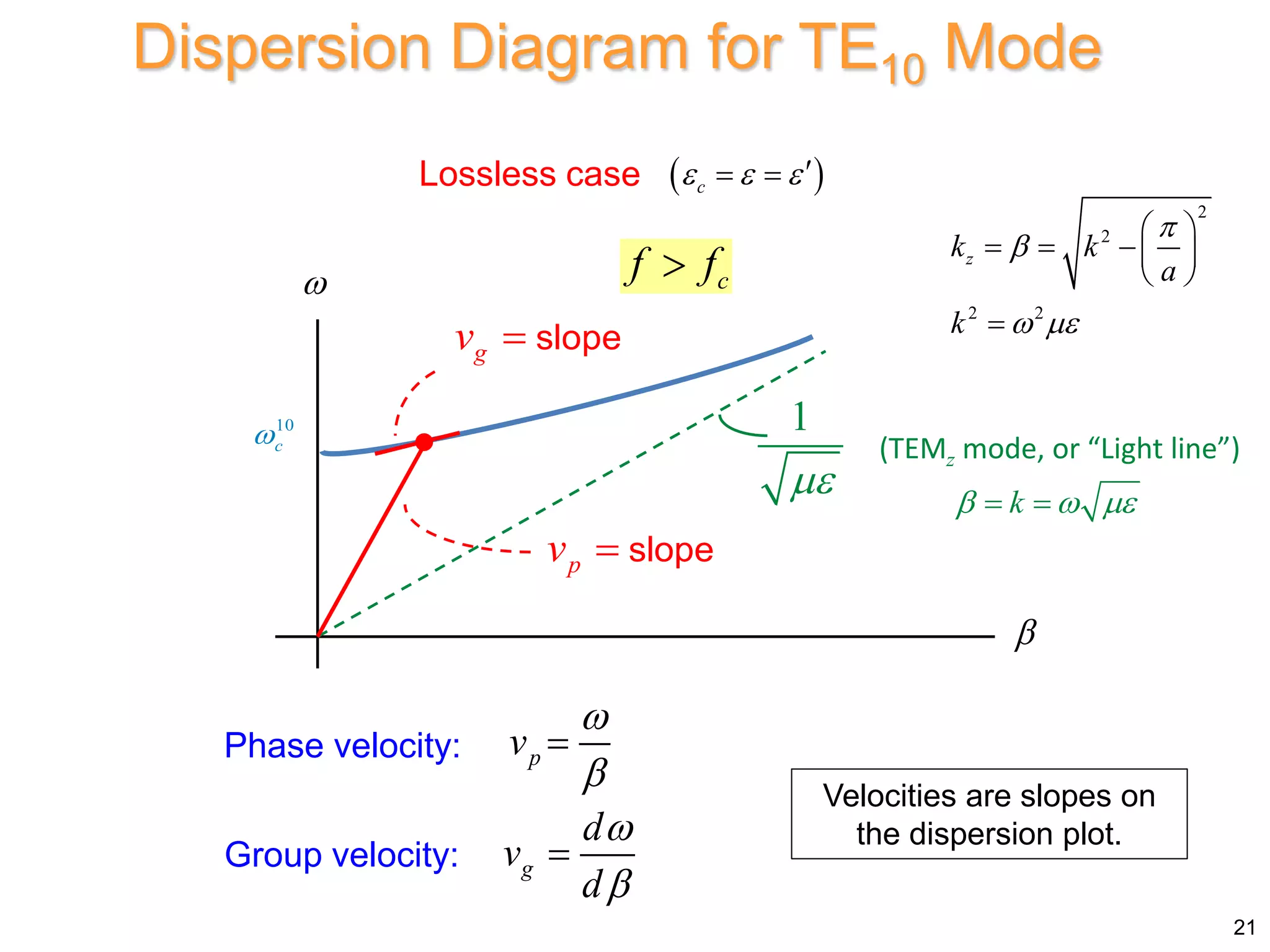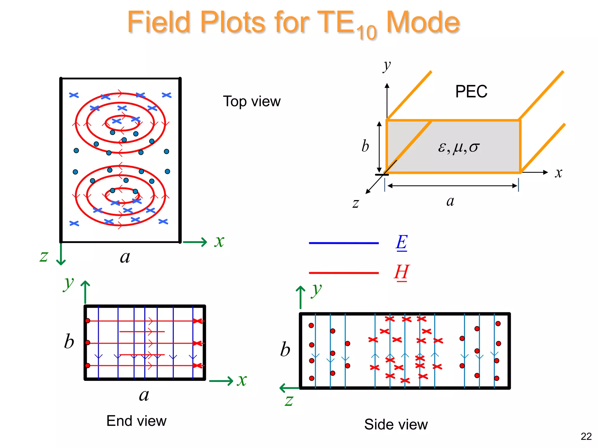3) The lowest frequency at which a mode can propagate is called the cutoff frequency. The dominant TE10 mode has the lowest cutoff frequency, allowing it to propagate over the widest frequency range.

1. Prof. David R. Jackson
Dept. of ECE
Notes 9
ECE 5317-6351
Microwave Engineering
Fall 2019
Waveguiding Structures Part 4:
Rectangular and Circular Waveguide
1
Adapted from notes by
Prof. Jeffery T. Williams

2.  One of the earliest waveguides.
 Still common for high power and low-
loss microwave / millimeter-wave
applications.
Rectangular Waveguide
 It is essentially an electromagnetic pipe
with a rectangular cross-section.
Single conductor No TEM mode
For convenience:
 a  b (the long dimension lies along x).
2

3. Rectangular Waveguide (cont.)
3
x
y
z a
b
PEC
, ,
  
0
1
(1 tan )
(1 tan )
c
c c
c
c
c
c d
r d
j
j j
j
j
j
j

 


 

 



 
  
 
 
  
 
 

 

 
 

 

 
 
Two types of modes:
TEz , TMz
 
1/2
2 2
z c
k k k
 
 
0 1 tan
c r d
k k j
   
  
2 2
2 2
:
:
c z c
c z c
f f k k k
f f k j k k
  
   
We need to solve for kc.
The cutoff wavenumber kc is real.

4.  
2 2
2
2 2
, 0
c z
k h x y
x y
 
 
  
 
 
 
For +z propagation:
   
, , , z
jk z
z z
H x y z h x y e

where
0 0
z
x
H
E
y

  

Subject to B.C.’s:
0 0
z
y
H
E
x

  

@ 0,
y b

@ 0,
x a

TEz Modes
 
1/2
2 2
c z
k k k
 
4
2
2
z z
x z
c
z z
y z
c
E H
j
E k
k x y
E H
j
E k
k y x


 
 

 
 
 
 
 
 
  
 
 
 
From previous field table:
x
y
z a
b
PEC
, ,
  

5.    
2 2
2
2 2
, ,
z c z
h x y k h x y
x y
 
 
  
 
 
 
Using separation of variables, let      
,
z
h x y X x Y y

2 2
2
2 2 c
d X d Y
Y X k XY
dx dy
   
2 2
2
2 2
1 1
c
d X d Y
k
X dx Y dy
   
2 2
2 2
2 2
1 1
x y
d X d Y
k k
X dx Y dy
    
and
Must be a constant
where “separation equation”
TEz Modes (cont.)
2 2 2
x y c
k k k
 
(eigenvalue problem)
5
(If we take one term across the equal sign, we
have a function of x equal to a function of y.)
This is the
“separation
equation”.

6. Hence,
 
( ) ( )
, ( cos sin )( cos sin )
X x Y y
z x x y y
h x y A k x B k x C k y D k y
  
Boundary Conditions:
0
z
h
y



0
z
h
x



@ 0,
y b

@ 0,
x a

0 0,1,2,...
y
n
D k n
b

   
and
0 0,1,2,...
x
m
B k m
a

   
and
 
2 2
2
, cos cos
z mn c
m x n y m n
h x y A k
a b a b
   
       
  
       
       
and
B
A
A
B
TEz Modes (cont.)
6

7. Therefore,
 
, , cos cos z
jk z
z mn
m n
H x y z A x y e
a b
  
   
    
   
 
1/2
2 2
1/2
2 2
2
z c
k k k
m n
k
a b
 
 
 
   
  
 
   
 
   
 
2
2
2
2
cos sin
sin cos
sin cos
cos sin
z
z
z
z
jk z
x mn
c
jk z
y mn
c
jk z
z
x mn
c
jk z
z
y mn
c
j n m n
E A x y e
k b a b
j m m n
E A x y e
k a a b
jk m m n
H A x y e
k a a b
jk n m n
H A x y e
k b a b
   
   
  
  




   
    
   
   
     
   
   
    
   
   
    
   
From the field table, we obtain the following:
But m = n = 0
is not allowed!
(non-physical solution)
Note:
00
ˆ ; 0
jkz
H z A e H

  
7
TEz Modes (cont.)
2 2
c
m n
k
a b
 
   
 
   
   
0,1,2,
0,1,2,
m
n



8. 8
TEz Modes (cont.)
Reason for non-physical solution
  2
0
H k H
    Vector wave equation: from Maxwell’s equations.
Take divergence of both sides.
Magnetic Gauss law
 
  2
0
H k H
      The divergence of a curl is zero.
0
H
 
Start with the vector wave equation:

9. 9
TEz Modes (cont.)
Revisit how we obtained the vector Helmholtz equation:
  2
0
H k H
   
0
H
 
Vector wave equation: from Maxwell’s equations.
  2 2
0
H
H H k H

     From definition of vector Laplacian
Magnetic Gauss law
2 2
0
H k H
   Vector Helmholtz equation (what we have solved)
Now use:
Reason for non-physical solution
A needed assumption!

10. 10
TEz Modes (cont.)
Reason for non-physical solution
Vector wave equation  magnetic Gauss law
The vector Helmholtz equation does not guarantee that the magnetic Gauss
law is satisfied. In the mathematical derivation, we need to assume the
magnetic Gauss law in order to arrive at the vector Helmholtz equation.
Note: The TE00 mode is the only one that violates the magnetic Gauss law.
Vector Helmholtz equation  magnetic Gauss law
All of the modes that we get by solving the Helmholtz equation should be
checked to make sure that they do satisfy the magnetic Gauss law.

11.  
 
1/2
2 2
1/2
2
2 2
mn mn
z c
m n
k k k k
a b
 
 
   
    
 
   
 
   
 
 TEmn mode is at cutoff when mn
c
k k

Lossless case
2 2
1
2
mn
c
m n
f
a b

   
 
   
   
Lowest cutoff frequency is for TE10 mode (a > b)
10 1
2
c
f
a 
 Dominant TE mode
(lowest fc)
We will
revisit this
mode later.
 
c
  
 
11
TEz Modes (cont.)
 
mn
c
k  


12. At the cutoff frequency of the TE10 mode (lossless waveguide):
10
2
1
2
d d d
d
c
c c c
a
f f
a


   
12
TEz Modes (cont.)
so
/ 2
c
d f f
a  


13. To have propagation:
c
f f

Example: Air-filled waveguide, f = 10 GHz. We have that a > 3.0 cm / 2 = 1.5 cm.
13
TEz Modes (cont.)
so
1
2
f
a 

1 1
2 2
2
d d
c
a
f
f


  
2
d
a


or
or

14. Recall:
   
, , , z
jk z
z z
E x y z e x y e

where
   
2 2
2
2 2
, ,
z c z
e x y k e x y
x y
 
 
  
 
 
 
 
1/2
2 2
c z
k k k
 
Subject to B.C.’s: 0
z
E  @ 0,
x a

@ 0,
y b

Thus, following same procedure as before, we have the following result:
TMz Modes
(eigenvalue problem)
14
x
y
z a
b
PEC
, ,
  

15.  
( ) ( )
, ( cos sin )( cos sin )
X x Y y
z x x y y
e x y A k x B k x C k y D k y
  
Boundary Conditions: 0
z
e  @ 0,
y b

@ 0,
x a

0 0,1,2,...
y
n
C k n
b

   
and
0 0,1,2,...
x
m
A k m
a

   
and
2 2
2
sin sin
z mn c
m n m n
e B x y k
a b a b
   
       
  
       
       
and
B
A
A
B
TMz Modes (cont.)
15

16. Therefore
 
, , sin sin z
jk z
z mn
m n
E x y z B x y e
a b
  
   
    
   
2
2
2
2
sin cos
cos sin
cos sin
sin cos
z
z
z
z
jk z
c
x mn
c
jk z
c
y mn
c
jk z
z
x mn
c
jk z
z
y mn
c
j n m n
H B x y e
k b a b
j m m n
H B x y e
k a a b
jk m m n
E B x y e
k a a b
jk n m n
E B x y e
k b a b
   
   
  
  




   
    
   
   
     
   
   
     
   
   
    
   
From the field table, we obtain the following:
Note:
If either m or n is zero, the
field becomes a trivial one in
the TMz case.
16
TMz Modes (cont.)
1,2,3
1,2,3
m
n


 
1/2
2 2
1/2
2 2
2
z c
k k k
m n
k
a b
 
 
 
   
  
 
   
 
   
 
2 2
c
m n
k
a b
 
   
 
   
   

17. 2 2
1
2
mn
c
m n
f
a b

   
 
   
   
The lowest cutoff frequency is obtained for the TM11 mode
2 2
11 1 1 1
2
c
f
a b

   
 
   
   
(same as for
TE modes)
Lossless case  
c
  
 
 
2 2
2
2 2
mn mn
z c
m n
k k k k
a b
 
   
    
   
   
Dominant TM mode
(lowest fc)
17
TMz Modes (cont.)

18. The maximum bandwidth for
single-mode operation is 67%.
 
/ 2
b a

10
TE 01
TE 11
TE
11
TM
b < a / 2
f
20
TE
10
TE
Single mode operation
10
TE 20
TE
11
TE
11
TM
b > a / 2
f
Single mode operation
10
TE 01
TE
Mode Chart
Two cases are considered:
2 2
1
2
mn
c
m n
f
a b

   
 
   
   
18
Lossless case  
c
  
 
x
y
z a
b
PEC
, ,
  
2 1
0
BW
f f
f


0
f center frequency

19. Dominant Mode: TE10 Mode
For this mode we have
10 cos z
jk z
z
H A x e
a
 
 
  
 
10 sin z
jk z
z
x
k a
H j A x e
a



 
  
 
10
10 sin z
jk z
y
E
j a
E A x e
a
 


 
   
 
1/2
2
10 2
z z
k k k
a

 
 
  
 
 
 
 
 
10 10
A E
j a




0
x z y
E E H
  
10
1, 0, c
m n k
a

  
Hence we have
10 sin z
jk z
y
E E x e
a
 
 
  
 
19
x
y
z a
b
PEC
, ,
  

20. Dominant Mode: TE10 Mode (cont.)
10 cos z
jk z
z
H E x e
j a a
 


 
  
  
 
 
 
10
1
sin z
jk z
x
TE
H E x e
Z a
 
 
   
 
0
x z y
E E H
  
10 sin z
jk z
y
E E x e
a
 
 
  
 
20
x
y
z a
b
PEC
, ,
  
The fields can be put in terms of E10:
TE
z
Z
k


1/2
2
10 2
z z
k k k
a

 
 
  
 
 
 
 
 

21. 2
2
2 2
z
k k
a
k


 
 
   
 

Phase velocity:
Group velocity: g
d
v
d



1


10
c


p
v  slope
p
v



Dispersion Diagram for TE10 Mode
Lossless case  
c
  
 
c
f f

(TEMz mode, or “Light line”)
Velocities are slopes on
the dispersion plot.
g
v  slope
21
k
  
 

22. Top view
E
H
End view Side view
Field Plots for TE10 Mode
22
x
z a
y
x
a
b
z
y
b
x
y
z a
b
PEC
, ,
  

23. Top view
s
J
H
End view Side view
Field Plots for TE10 Mode (cont.)
23
x
z a
y
x
a
b
z
y
b
x
y
z a
b
PEC
, ,
  
Note: One can cut a narrow z-directed slot in the center of the top wall without disturbing the current.

24. Time-average power flow in the z direction for +z mode:
 
*
10
0 0
*
0 0
2 2
10
1
ˆ
Re
2
1
Re
2
1
Re
2 2
a b
a b
y x
z
z
P E H z dydx
E H dydx
ab k
E e 



 
  
 
 
 
 
 
 
 
 
 
  
   
   
 


Simplifying, we have
 
2 2
10 10
Re
4
z
z
ab
P k E e 

 
 
  
 
Note:
For a given maximum electric field level (e.g., the
breakdown field), the power is increased by increasing the
cross-sectional area (ab).
Power Flow for TE10 Mode
2
0 0
sin
2
a b
x ab
dydx
a

 

 
 

Note:
24
10 sin z
jk z
y
E E x e
a
 
 
  
 
10
1
sin z
jk z
x
TE
H E x e
Z a
 
 
   
 
TE
z
Z
k


At breakdown:
10 c
E E


25. From Notes 7 we have:
25
Dielectric Attenuation for TE10 Mode
2 2
2 2
2 2
2 2
0
2
0
Re
Im
tan
2
z d c
c
d c
r r c
r r d
d
k j k k
k k
k k
k k
k
 


  
  


   
 
  
 

0 1 tan
r r d
k k jk k j
  
 
    c
k
a


c
f f


26. Recall
0
(0)
2
l
c
P
P
 
2
(0)
2
s
l s
C
R
P J d
 
0 10 0
z
P P

 (calculated on previous slide)
ˆ
s
J n H
  on conductor
Conductor Attenuation for TE10 Mode
26
left right bot top
C C C C C
   
x
y
z a
b
s
R
Lossless

27. Side walls
left
10
0
right
10
ˆ ˆ ˆ
@ 0:
ˆ ˆ ˆ
@ :
z
z
jk z
s z
x
jk z
s z
x a
x J x H yH yA e
x a J x H yH yA e




     
      
Conductor Attenuation for TE10 Mode
left right
10
z
jk z
sy sy
J J A e
  
27
10
10
cos
sin
z
z
jk z
z
jk z
z
x
H A x e
a
k a
H j A x e
a





 
  
 
 
  
 
x
y
z a
b
s
R
Lossless
Hence:

28. Top and bottom walls
bot
0
top
ˆ
@ 0:
ˆ
@ :
s y
s y b
y J y H
y b J y H


  
   
(The fields of this mode are independent of y.)
Conductor Attenuation for TE10 Mode (cont.)
top bot
s s
J J
 
10
10
cos
sin
z
z
jk z
z
jk z
z
x
H A x e
a
k a
H j A x e
a





 
  
 
 
  
 
bot
10
bot
10
cos
sin
z
z
jk z
sx
jk z
z
sz
J A x e
a
k a
J j A x e
a





 
  
 
 
  
 
28
Hence:
x
y
z a
b
s
R
Lossless

29.  
2 2
left bot
0 0
2 2 2
left bot bot
0 0
2 2
2
10 10 10
0 0
2
2 2 2
10
(0) 2
2 2
cos sin
cos sin
b a
s s
l s s
b a
s sy s sx sz
b a
z
s s
z
s
R R
P J dy J dx
R J dy R J J dx
k a
R A dy R A x j A x dx
a a
k a
R A dy x dx x
a a
 

 

 
 
 
 
  
 
   
    
 
   
 
   
 
 
   
    
   
   
 
 
 
 
0 0 0
2 2
2
10 2
2 2
b a a
z
s
dx
k a
a a
R A b

 
 
 
 
 
  
 
 
 
  
Conductor Attenuation for TE10 Mode (cont.)
29
We then have:
x
y
z a
b
s
R
Lossless

30. 2 3
2
10 2
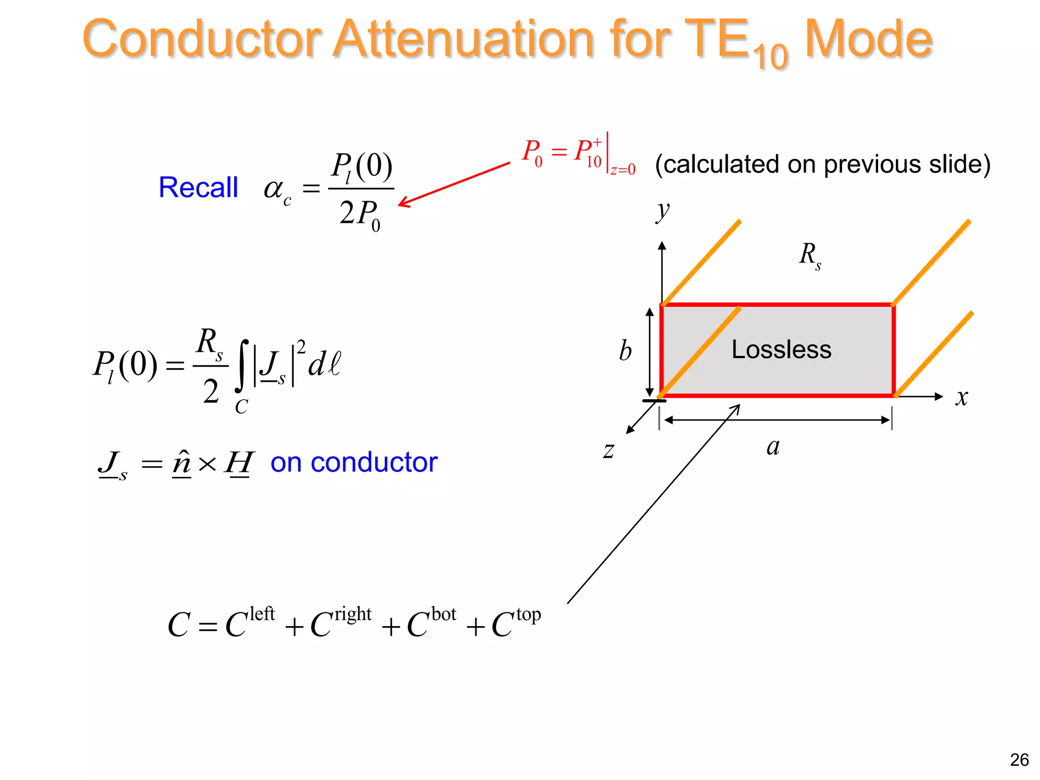
(0)
2 2
l s
a a
P R A b


 
  
 
 
 
 
2 3 2
3
2 [np/m]
s
c
R
b a k
a b k
 
 
 
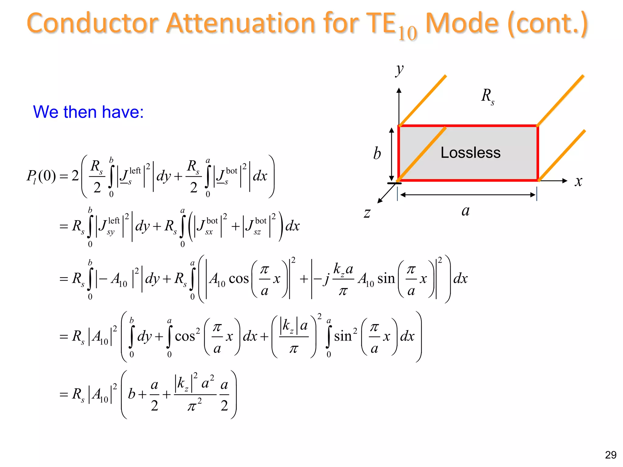
Attenuation for TE10 Mode (cont.)
2
0 10
4
ab
P E


 
  
 
0
(0)
2
l
c
P
P
 
Simplify, using 2 2 2
c
k k
  
10
c
k
a


Final result:
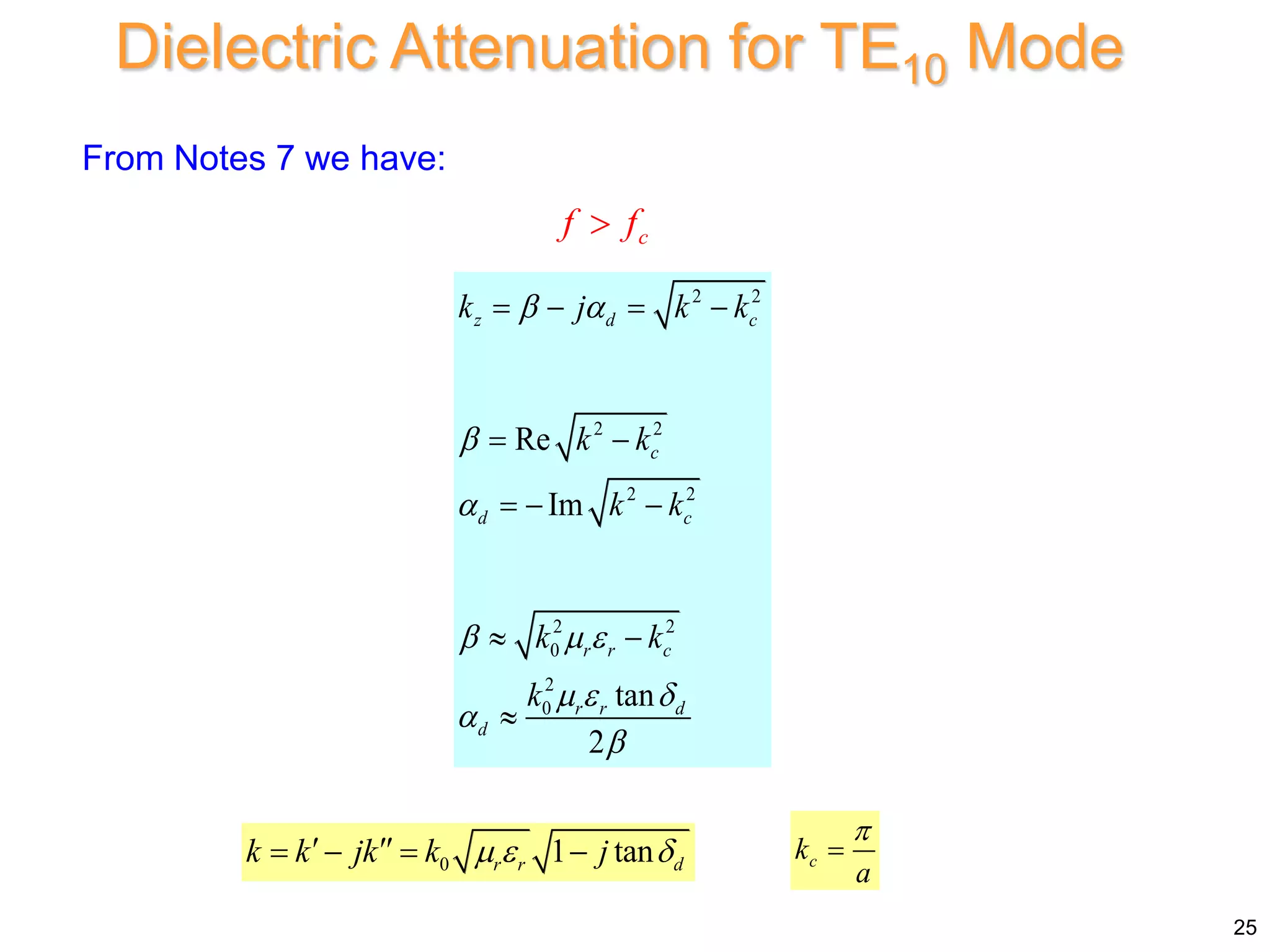
Assume f > fc
z
k 
 (The wavenumber is taken as that
of a guide with perfect walls.)
30
10 10
A E
j a




x
y
z a
b
s
R
Lossless

31.  
 
2 3 2
3
2 [np/m]
s
c
R
b a k
a b k
 
 
 
Attenuation for TE10 Mode (cont.)
31
x
y
z a
b
s
R
Lossless
 
2
2
1 2
1 [np/m]
1 /
s c
c
c
R f
b
b a f
f f


 
 
 
 
 
 
 
  
Two alternative forms for the
final result:
Final Formulas

32. Attenuation for TE10 Mode (cont.)
 
7
2.6 10 [S/m]
  
Brass X-band air-filled waveguide
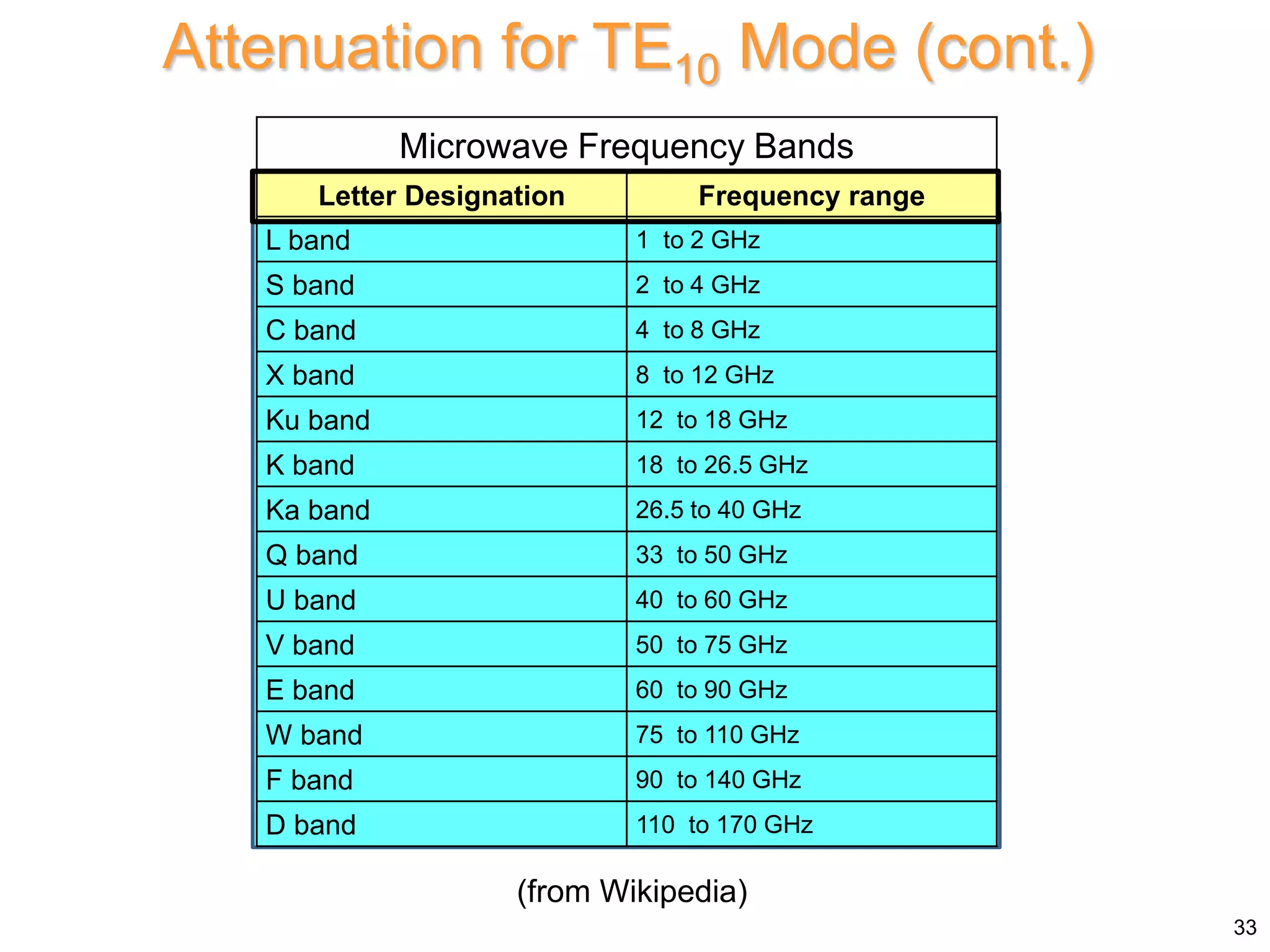
X : 8 12 [GHz]

band
(See the table on the next slide.)
32
a = 2.0 cm
(from the Pozar book)

33. Attenuation for TE10 Mode (cont.)
Microwave Frequency Bands
Letter Designation Frequency range
L band 1 to 2 GHz
S band 2 to 4 GHz
C band 4 to 8 GHz
X band 8 to 12 GHz
Ku band 12 to 18 GHz
K band 18 to 26.5 GHz
Ka band 26.5 to 40 GHz
Q band 33 to 50 GHz
U band 40 to 60 GHz
V band 50 to 75 GHz
E band 60 to 90 GHz
W band 75 to 110 GHz
F band 90 to 140 GHz
D band 110 to 170 GHz
(from Wikipedia)
33

34. 10
20
01
11
11
30
21
21
TE 6.55
TE 13.10
TE 14.71
TE 16.10
TM 16.10
TE 19.65
TE 19.69
TM 19.69
2.29cm (0.90in)
1.02cm (0.40in)
a
b


Mode fc [GHz]
X : 8 12 [ ]

band GHz
50 mil (0.05”) thickness
Modes in an X-Band Waveguide
“Standard X-band waveguide” (WR90)
34
a
b
1"
0.5"

35. Determine , , and g (as appropriate) at
10 GHz and 6 GHz for the TE10 mode in a
lossless air-filled X-band waveguide.
2 2
0.0397
158.25
g
 


  
2
2 2
10
2
8
2 10
2.99792458 10 0.0229
a
  
  
 
   
   
   
 

   
 
@ 10 GHz
Example: X-Band Waveguide
158.25 [rad/m]
 
3.97 [cm]
g
 
35
a = 2.29cm
b = 1.02cm
0 0
,
 
2 2 2
: 2
/
d d d d
f
k f
c f c c
   
   

     
Lossless

36. 1/2
1/2 2
2 2
9
2
8
2
2 9
8
2 6 10
2.99792458 10 0.0229
2 6 10
0.0229 2.99792458 10
55.04 [1/m]
z
k
a
j
j
  
 
 
 
   

   
   
 
 
   
 
   

   
 
   
 

 
  
   

   
 
2
g




Evanescent mode:  = 0; g is not defined!
@ 6 GHz
Example: X-Band Waveguide (cont.)
55.04 [np/m]
478.08 [dB/m]
 

36

37. Fields of a Guided Wave
37
2
2
2
2
c z z
z
c
z z z
c
c
z z
z
c
z z z
c
E H
j
H k
k
E k H
j
H
k y
E H
j
E k
k
k E H
j
E
k





  

 

  

  
 
 
  
 
 
 
 

 
 
 
 
 
 

  
 
 
 
 
 
 
 
 
 
Fields Equations in Cylindrical Coordinates
These equations give the transverse
field components in terms of the
longitudinal components, Ez and Hz.
2 2
c
k  

2 2
c z
k k k
 
  z
jk z
F z e

These are useful for a circular waveguide.

38. Circular Waveguide
TMz mode:
   
2 2
, ,
z c z
e k e
   
  
2 2 2
z c
k k k
 
The solution in cylindrical coordinates is:
 
( ) sin( )
,
( ) cos( )
n c
z
n c
J k n
e
Y k n
 
 
 
   
    
 
 
Note: The value n must be an integer to have unique fields.
38
(eigenvalue problem)
PEC
a
z
, ,
  
This means any combination of
these two functions.

39. 39
References for Bessel Functions
 M. R. Spiegel, Schaum’s Outline Mathematical Handbook, McGraw-Hill, 1968.
 M. Abramowitz and I. E. Stegun, Handbook of Mathematical Functions with
Formulas, Graphs, and Mathematical Tables, National Bureau of Standards,
Government Printing Office, Tenth Printing, 1972.
 N. N. Lebedev, Special Functions & Their Applications, Dover Publications, New
York, 1972.
( )
( )
n
n
J x n
Y x n


Bessel function of the first kind of order
Bessel function of the secondkind of order
References:

40. Plot of Bessel Functions
0 1 2 3 4 5 6 7 8 9 10
0.6
0.4
0.2
0
0.2
0.4
0.6
0.8
1
1
0.403

J0 x
( )
J1 x
( )
Jn 2 x

( )
10
0 x
x
Jn (x)
n = 0
n = 1
n = 2
(0)
n
J is finite
2
( ) ~ cos ,
2 4
n
n
J x x x
x
 

 
   
 
 
1
( ) ~ 0,1,2,...., 0
2 !
n
n n
J x x n x
n
 
 
 
 
40

41. Plot of Bessel Functions (cont.)
0 1 2 3 4 5 6 7 8 9 10
7
6
5
4
3
2
1
0
1
0.521
6.206

Y0 x
( )
Y1 x
( )
Yn 2 x

( )
10
0 x
x
Yn (x)
n = 0
n = 1
n = 2
(0)
n
Y is infinite
2
( ) ~ sin ,
2 4
n
n
Y x x x
x
 

 
   
 
 
0
2
( ) ~ ln , 0.5772156, 0
2
x
Y x x
 

 
 
  
 
 
 
 
1 2
( ) ~ ( 1)! , 1,2,3,....., 0
n
n
Y x n n x
x

 
   
 
  41

42. Circular Waveguide (cont.)
Choose (somewhat arbitrarily) cos( )
n
 
( )
, cos( )
( )
n c
z
n c
J k
e n
Y k

  

 
  
 
The field should be finite on the z axis.
( )
n c
Y k  is not allowed
 
, , cos( ) ( ) z
jk z
z n c
E z n J k e
    

42
 
, cos( ) ( )
z n c
e n J k
   

Hence, we have

43. B.C.’s:  
, , 0
z
E a z
 
Circular Waveguide (cont.)
( ) 0
n c
J k a 
Hence
c np
k a x
 np
c
x
k
a

Note: The value xn0 = 0 is not included
since this would yield a trivial solution:  
0 0 0
n n n
J x J
a

 
 
 
 
43
(This is true unless n = 0, in which
case we cannot have p = 0.)
Sketch for a typical value of n (n  0).
Note: Pozar uses the notation pmn.
x
( )
n
J x
1
n
x 2
n
x
3
n
x

44. TMnp mode:
 
, , cos( ) 0,1,2
z
jk z
z n np
E z n J x e n
a

   
 
 
 
 
2
2
1,2,3,.........
np
z
x
k k p
a
 
  
 
 
Circular Waveguide (cont.)
44

45. Cutoff Frequency: TMz
np
c
x
k k
a
 
TM
2 np
c
x
f
a
  
TM
2
d
c np
c
f x
a

 
  
 
0
z
k 
2 2 2
z c
k k k
 
At f = fc :
d
r
c
c


45
Assume k is real here.

46. Cutoff Frequency: TMz (cont.)
TM01, TM11, TM21, TM02, ……..
p n 0 1 2 3 4 5
1 2.405 3.832 5.136 6.380 7.588 8.771
2 5.520 7.016 8.417 9.761 11.065 12.339
3 8.654 10.173 11.620 13.015 14.372
4 11.792 13.324 14.796
xnp values
46

47. TEz Modes
 
, , cos( ) ( ) z
jk z
z n c
H z n J k e
    

Proceeding as before, we now have that
Set  
, , 0
E a z
  
1 z
c
H H
E
j z


 

 

 
 
 
 
0
a
z
H

 

 

(From Ampere’s law)
( ) 0
n c
J k a
 
Hence
47
The prime denotes derivative
with respect to the argument.
 
0
a
H





48. 1,2,3,.....
c np
np
c
k a x
x
k p
a



 
( ) 0
n c
J k a
 
TEz Modes (cont.)
We don’t need to consider p = 0;
this is explained on the next slide.
48
Sketch for a typical value of n (n  1).
x
( )
n
J x

1
n
x 2
n
x
3
n
x

49. TEz Modes (cont.)
 
, , cos( ) 1,2,
z
jk z
z n np
H z n J x e p
a

   
 

 
 
 
Note: If p = 0, then 0
np
x 
 
0 0
n np n
J x J
a

 
  
 
 
(trivial solution)
0
n 
0
n   
0 0 0 1
np
J x J
a

 
  
 
 
ˆ ˆ
z z
jk z jk z jkz
z
H e H z e H z e
  
      (nonphysical solution)
We then have, for p = 0:
The TE00 mode is not physical.
49
(violates the magnetic Gauss law)

50. TEnp mode:
 
, , cos( ) 0,1,2
z
jk z
z n np
H z n J x e n
a

   
 

 
 
 
2
2
1,2,3,.........
np
z
x
k k p
a

 
  
 
 
Circular Waveguide (cont.)
50

51. Cutoff Frequency: TEz
np
c
x
k k
a

 
2 np
TE
c
x
f
a
 


2
TE d
c np
c
f x
a

 

  
 
0
z
k 
2 2 2
z c
k k k
 
Hence
d
r
c
c


51
Assume k is real here.

52. TE11, TE21, TE01, TE31, ……..
p n 0 1 2 3 4 5
1 3.832 1.841 3.054 4.201 5.317 5.416
2 7.016 5.331 6.706 8.015 9.282 10.520
3 10.173 8.536 9.969 11.346 12.682 13.987
4 13.324 11.706 13.170
x´np values
Cutoff Frequency: TEz
52

53. TE11 Mode
TE10 mode of
rectangular waveguide
TE11 mode of
circular waveguide
The dominant mode of circular waveguide is the TE11 mode.
The TE11 mode can be thought of as an evolution of the TE10 mode of
rectangular waveguide as the boundary changes shape.
Electric field
Magnetic field
(From Wikipedia)
53

54. TE11 Mode (cont.)
The attenuation due to conductor loss for the TE11 mode is:
54
The derivation is in the Pozar book (see Eq. 3.133).
 
2
2
2
11
1 1
1
1 /
s c
c
c
R f
a f x
f f


 
 
 
 
 
 
 
 
  
11 1.841
x 
11
c
x
k
a



55. TE01 Mode
The TE01 mode of circular waveguide has the unusual property that the
conductor attenuation decreases with frequency. (With most waveguide
modes, the conductor attenuation increases with frequency.)
The TE01 mode was studied extensively as a candidate for long-range
communications – but eventually fiber-optic cables became available with
even lower loss. It is still useful for some high-power applications.
55
Note: This mode is not the dominant mode!
Reason: This mode has current only in the  direction, and this component of current
(corresponding to Hz) decreases as the frequency increases (for a fixed power flow
down the guide, i.e., a fixed E). (Please see the equations on the next slide.)
 
 
01
2
TE
2
/
1 /
c
s
c
c
f f
R
a f f





56. TE01 Mode (cont.)
56
 
0 01
01
0 01
2
0,1
1
/
z
z
jk z
z
jk z
c
TE
H J x e
a
x
E j J x e
a k a
H E Z

 





 

  
 

   
 
  
 
 
 
 
The fields of the TE01 mode are:
 
 
0,1
0,1
TE
z
Z
k



57. TE01 Mode (cont.)
57
0
(0)
2
l
c
P
P
 
Note: P0 = 0 at cutoff
c

f
11
TE
c
f 01
TM
c
f 21
TE
c
f 01
TE
c
f
11
TE 01
TM 21
TE
11
TM
01
TE
Note: The attenuation increases at high frequency for all other modes, due to Rs.

58. TE01 Mode (cont.)
Practical Note:
The TE01 mode has only an azimuthal ( - directed) surface current on the
wall of the waveguide. Therefore, it can be supported by a set of conducting
rings, while the lower modes (TE11 ,TM01, TE21, TM11) will not propagate on
such a structure.
(A helical spring will also work fine.)
58
E
H
TE01 mode:

59. 59
Products include:
4-Port Diplexers, CP or Linear;
3-Port Diplexers, 2xRx & 1xTx;
2-Port Diplexers, RxTx, X-Pol or
Co-Pol, CP or Linear;
TE21 Monopulse Tracking Couplers;
TE01 Mode Components; Transitions;
Filters; Flex Waveguides;
Waveguide Bends; Twists; Runs; etc.
Many of the items are "off the shelf products".
Products can be custom tailored to a customer's
application.
Many of the products can be supplied with standard
feed horns for prime or offset antennas.
VertexRSI's Torrance Facility is a leading supplier of antenna feed components for the
various commercial and military bands. A patented circular polarized 4-port diplexer
meeting all Intelsat specifications leads a full array of products.
TE01 Mode (cont.)

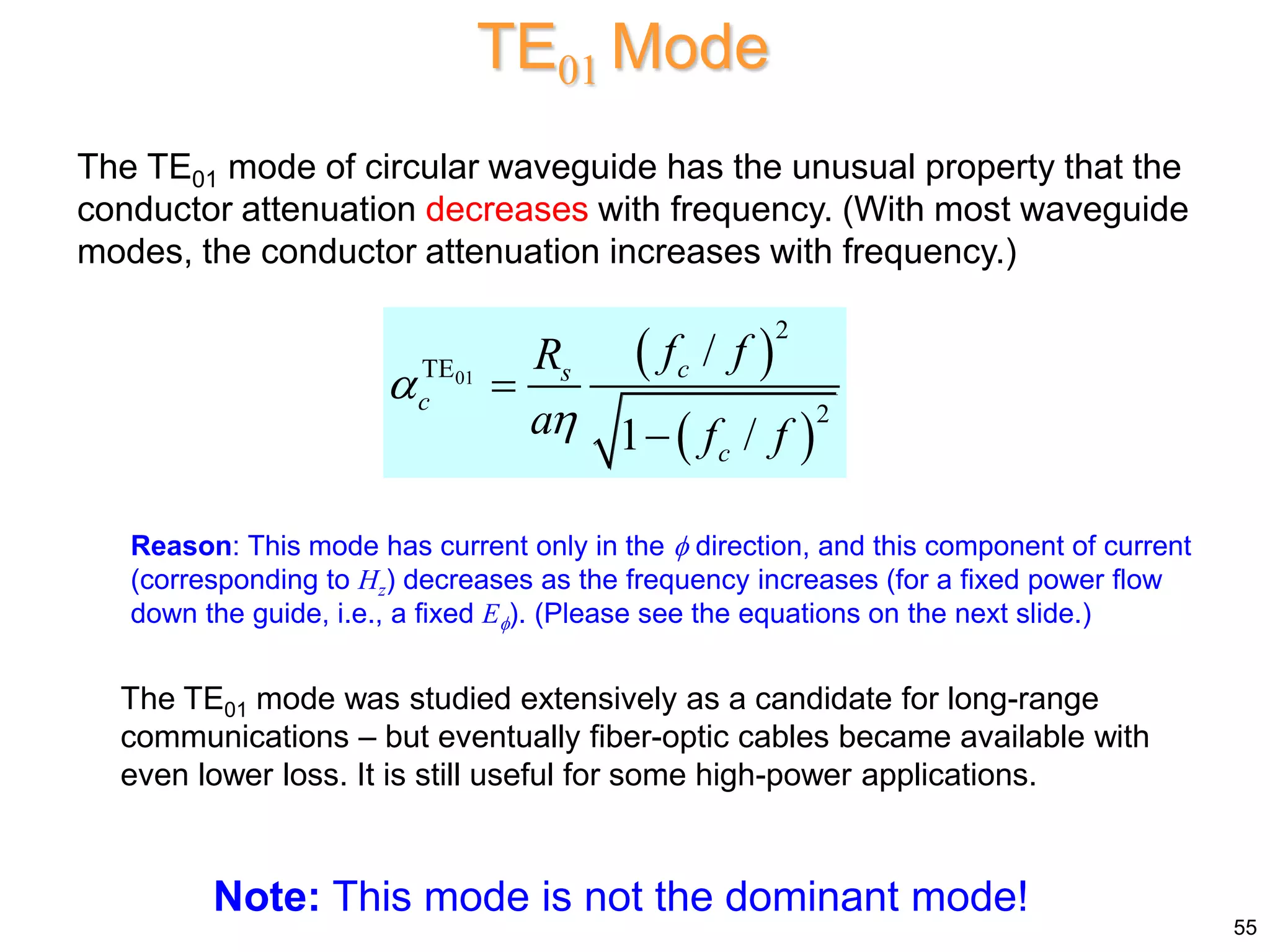
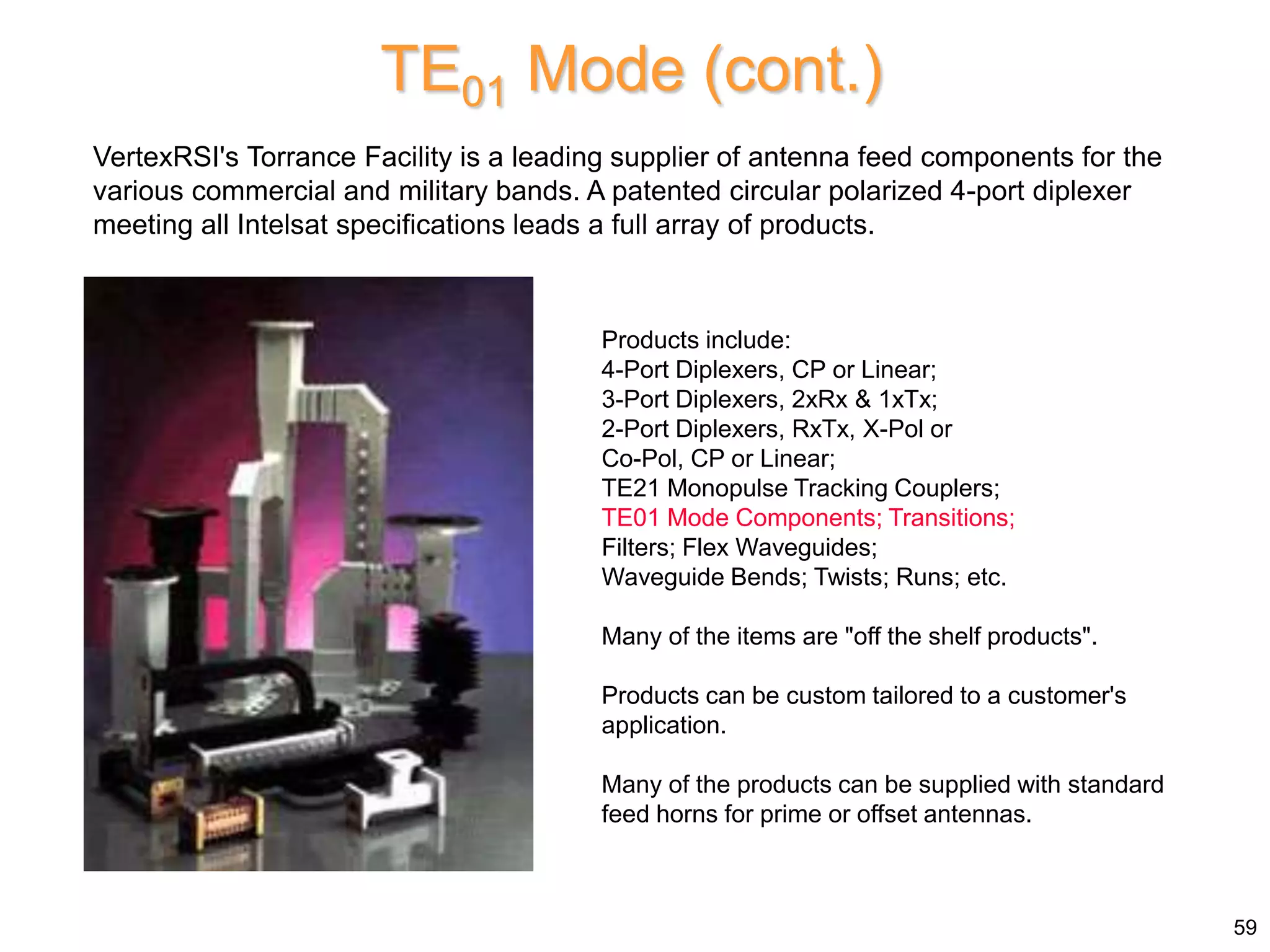
60. From the beginning, the most obvious application of waveguides had been as a
communications medium. It had been determined by both Schelkunoff and Mead,
independently, in July 1933, that an axially symmetric electric wave (TE01) in circular
waveguide would have an attenuation factor that decreased with increasing frequency
[44]. This unique characteristic was believed to offer a great potential for wide-band,
multichannel systems, and for many years to come the development of such a system
was a major focus of work within the waveguide group at BTL. It is important to note,
however, that the use of waveguide as a long transmission line never did prove to be
practical, and Southworth eventually began to realize that the role of waveguide would
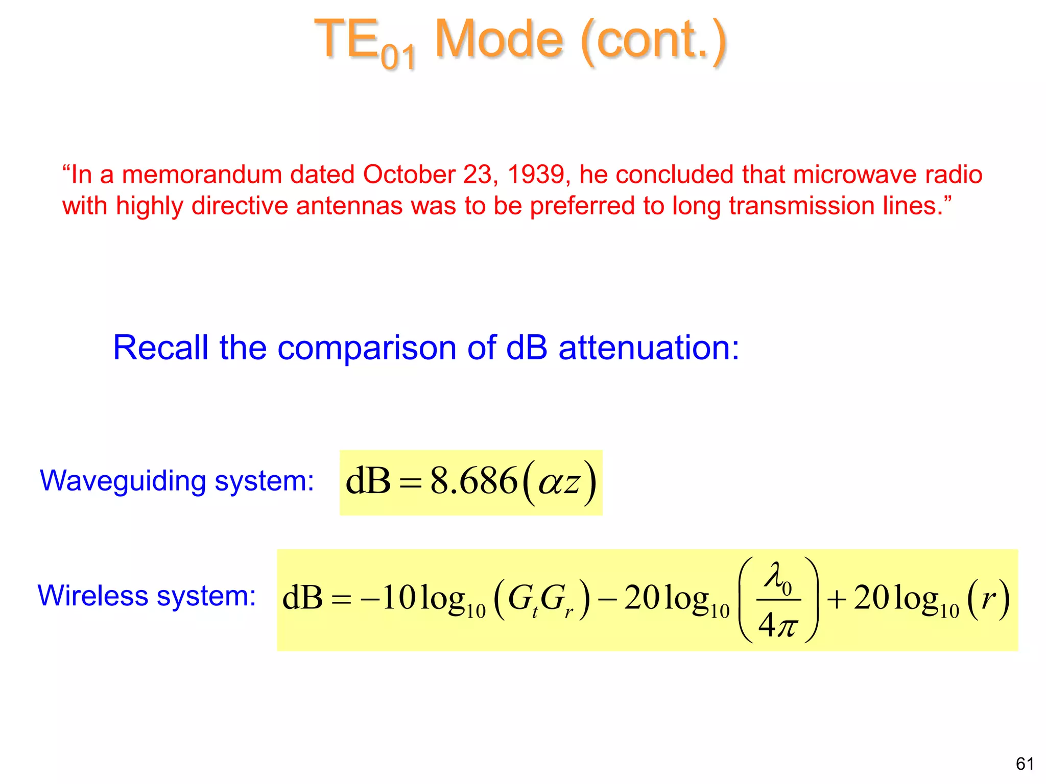
be somewhat different than originally expected. In a memorandum dated October 23,
1939, he concluded that microwave radio with highly directive antennas was to be
preferred to long transmission lines. "Thus," he wrote, “we come to the conclusion that
the hollow, cylindrical conductor is to be valued primarily as a new circuit element, but
not yet as a new type of toll cable” [45]. It was as a circuit element in military radar that
waveguide technology was to find its first major application and to receive an enormous
stimulus to both practical and theoretical advance.
K. S. Packard, “The origins of waveguide: A case of multiple rediscovery,” IEEE Trans.
Microwave Theory and Techniques, pp. 961-969, Sept. 1984.
TE01 Mode (cont.)
60

61. 61
Waveguiding system:  
dB 8.686 z


Wireless system:    
0
10 10 10
dB 10log 20log 20log
4
t r
G G r


 
   
 
 
Recall the comparison of dB attenuation:
TE01 Mode (cont.)
“In a memorandum dated October 23, 1939, he concluded that microwave radio
with highly directive antennas was to be preferred to long transmission lines.”