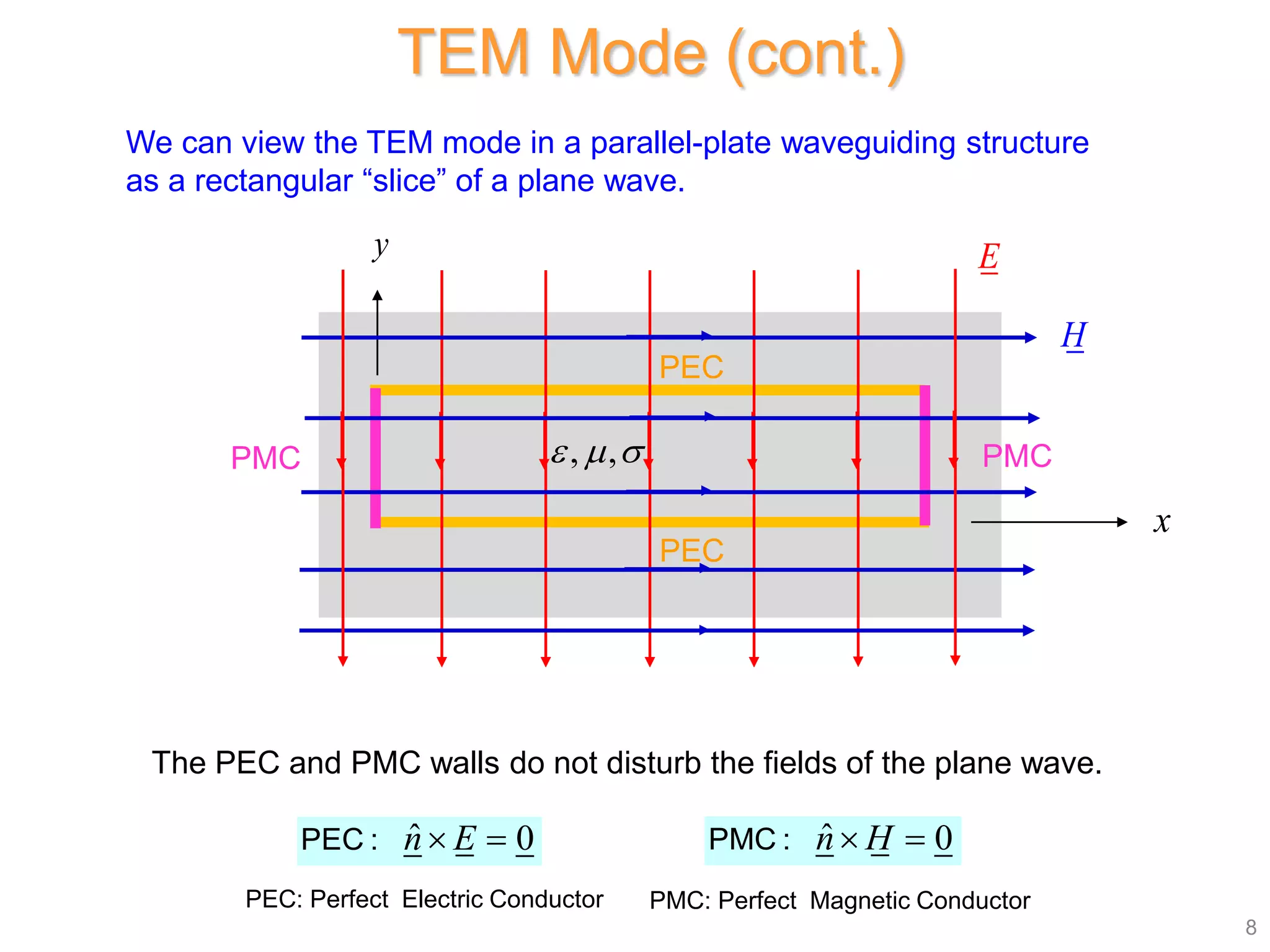
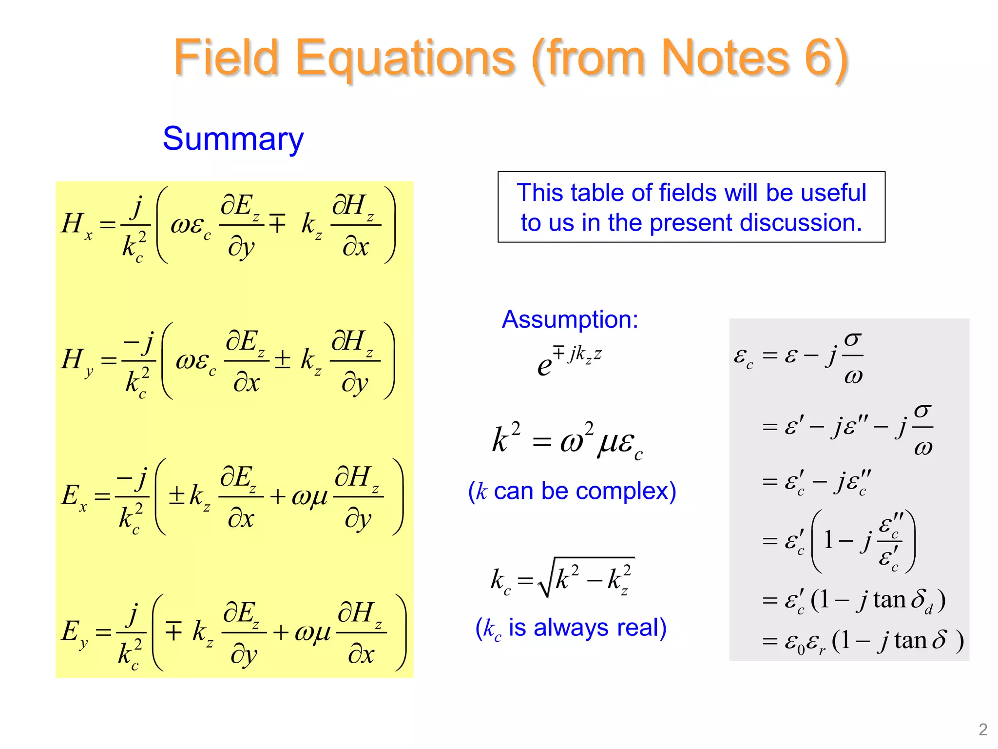
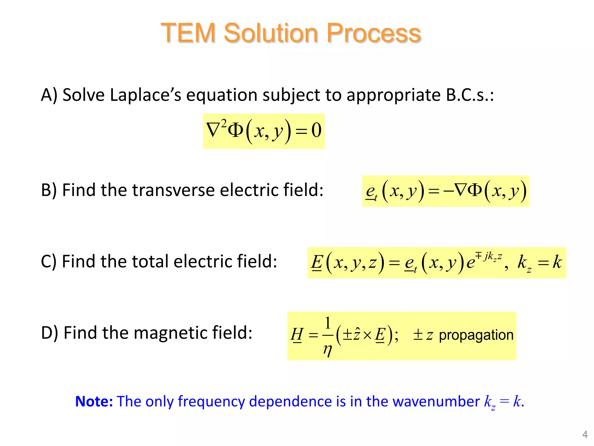
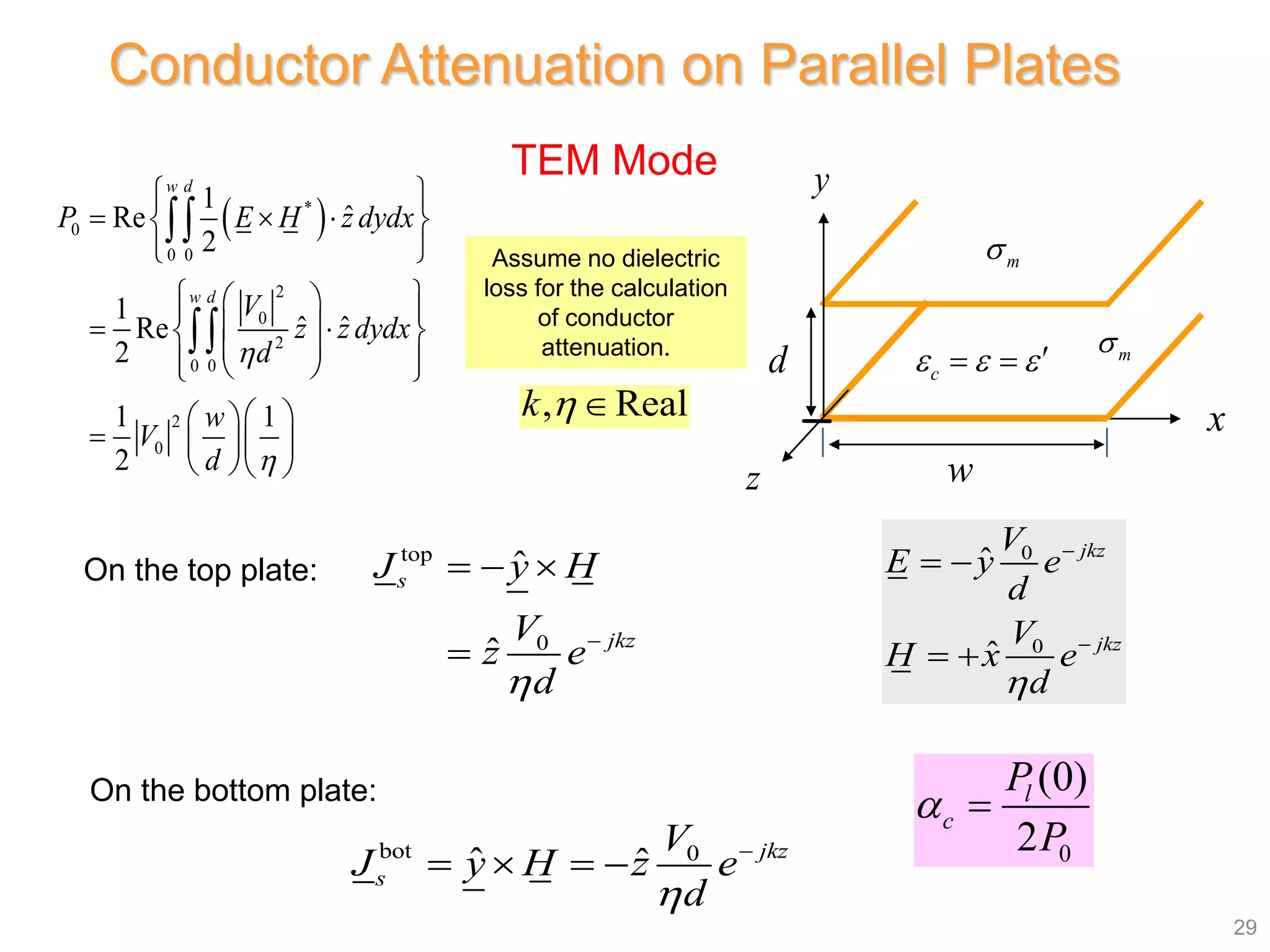
- The document discusses the transverse electromagnetic (TEM) mode in a parallel-plate waveguide structure. - A TEM mode can propagate between the parallel plates, with the electric and magnetic fields confined between the plates. The fields are independent of the propagation direction z. - Expressions are derived for the voltage, current, characteristic impedance, and power flow of the TEM transmission line mode between the plates. 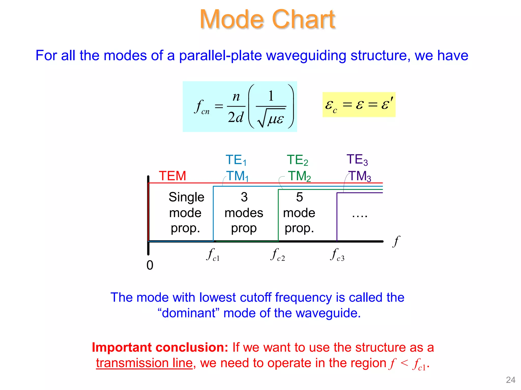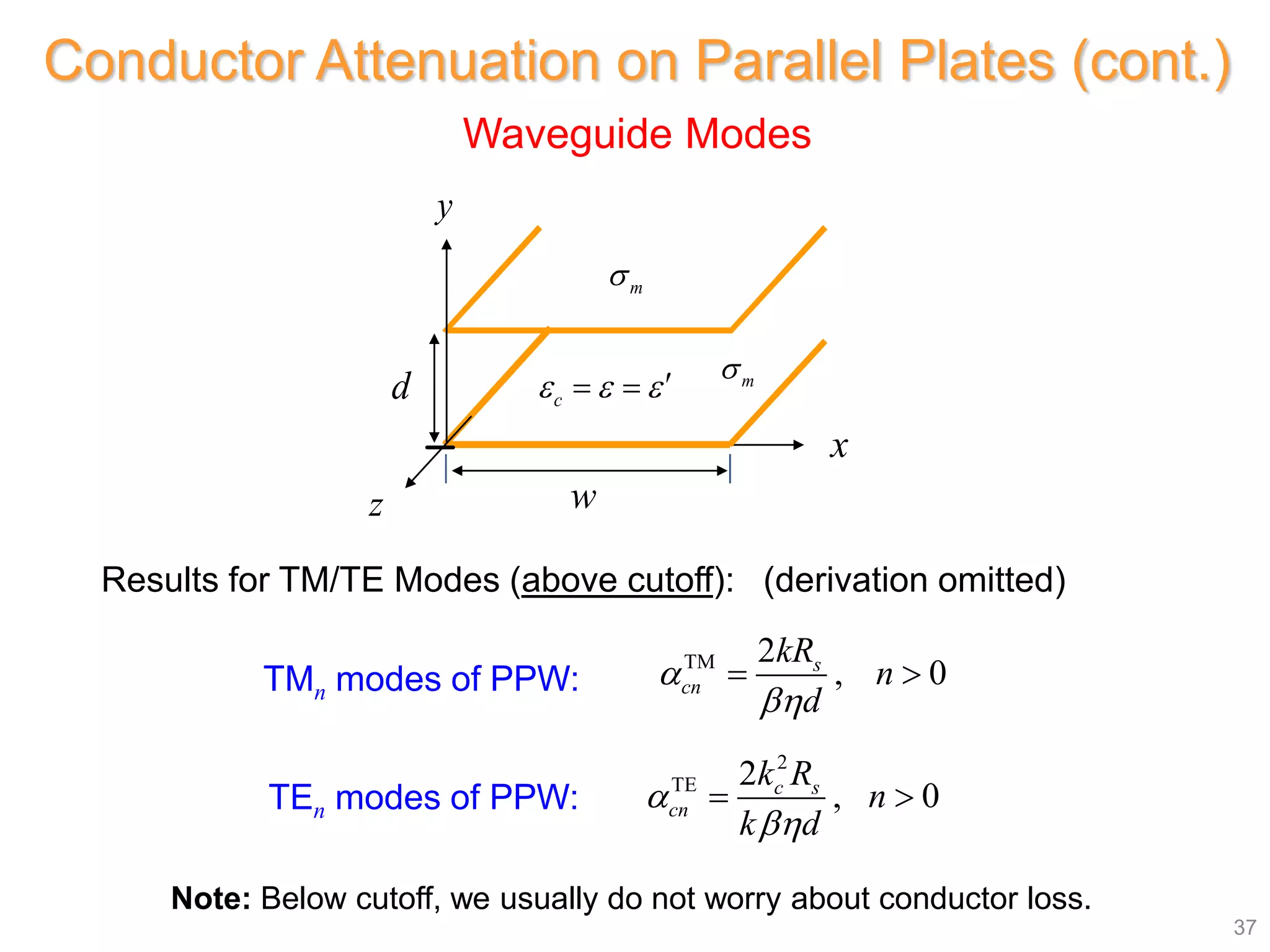- Higher order transverse magnetic (TM) modes are also possible, where the magnetic field has only a z-component. The eigenvalue equation for these modes is presented.

1. Prof. David R. Jackson
Dept. of ECE
Notes 8
ECE 5317-6351
Microwave Engineering
Fall 2019
Waveguiding Structures
Part 3: Parallel Plates
1
, ,
  
x
z
y
d
w
Adapted from notes by
Prof. Jeffery T. Williams

2. 2
2
2
2
z z
x c z
c
z z
y c z
c
z z
x z
c
z z
y z
c
E H
j
H k
k y x
E H
j
H k
k x y
E H
j
E k
k x y
E H
j
E k
k y x




 
 
  
 
 
 
 

 
 
 
 
 
 

  
 
 
 
 
 
 
 
 
 
Summary
2 2
c
k  

2 2
c z
k k k
 
Field Equations (from Notes 6)
This table of fields will be useful
to us in the present discussion.
2
(kc is always real)
(k can be complex)
z
jk z
e
0
1
(1 tan )
(1 tan )
c
c c
c
c
c
c d
r
j
j j
j
j
j
j

 


 

 



 
  
 
 
  
 
 

 

 
 

 

 
 
Assumption:

3. Parallel-Plate Waveguiding Structure
 Both plates assumed PEC
 w >> d
0
x

 

The parallel-plate structure is a good approximate model for a wide microstrip line.
3
(neglect edge effects)
,
w
h
, ,
  
c j

 

 
, ,
  
x
z
y
d
w
PEC

4. 4
TEM Solution Process
A) Solve Laplace’s equation subject to appropriate B.C.s.:
B) Find the transverse electric field:
C) Find the total electric field:
D) Find the magnetic field:
 
2
, 0
x y
  
 
1
ˆ ;
H z E z

    propagation
   
, ,
t
e x y x y
 
   
, , , ,
z
jk z
t z
E x y z e x y e k k
 
Note: The only frequency dependence is in the wavenumber kz = k.

5. 2 conductors  1 TEM mode
To solve for TEM mode:
 
2
, 0
x y
  
Boundary conditions:
0
( ,0) 0 ; ( , )
x x d V
   
2 2
2
2 2
0
x y
 
 
     
 
 
 
TEM Mode
z c
k j k k jk
     
     
k
k






5
0
0
x w
y d
 
 
, ,
  
x
z
y
d
w
PEC

6. where
( , )
x y A By
  
0
ˆ
( , , ) ( , ) jkz jkz
t
V
E x y z e x y e y e
d
  
0
A 
2
2
0
y
 


    0
,0 0 & ,
x x d V
   
  0
ˆ ˆ
,
t
V
e x y y y
y d

      

TEM Mode (cont.)
6
0
V
B
d

0
( , )
V
x y y
d
 
Hence
We then have

7. Recall
  0
ˆ
, , jkz
V
H x y z x e
d

  
1
ˆ
( )
H z E

  
0
ˆ
( , , ) jkz
V
E x y z y e
d
 
TEM Mode (cont.)
7
c




c j

 

 
Fields for +z mode: E
H
x
y
0
V
, ,
  
, ,
  
x
z
y
d
w
PEC

8. TEM Mode (cont.)
8
We can view the TEM mode in a parallel-plate waveguiding structure
as a rectangular “slice” of a plane wave.
The PEC and PMC walls do not disturb the fields of the plane wave.
ˆ 0
n E
 
PEC : ˆ 0
n H
 
PMC :
PEC
PEC
PMC
PMC , ,
  
x
E
H
y
PEC: Perfect Electric Conductor PMC: Perfect Magnetic Conductor

9. Assume a wave propagating the
in + z direction henceforth.
Time-ave power flow in + z direction:
 
*
2
0 2
* 2
0 0
2 2
0 2 *
1
ˆ
Re ( )
2
1
ˆ ˆ
Re
2
1 1 1
Re
2
s
w d
k z
k z
P E H z dS
V
z z e dydx
d
V wd e
d







 
  
 
 
 
 
 
  
 
 
 
 
 
 
 
    
   


2 2
0 *
1 1
Re
2
k z
w
P V e
d 

 
 
 
    
   
TEM Mode (cont.)
9
 
0
0
ˆ
( , , )
ˆ
, ,
jkz
jkz
V
E x y z y e
d
V
H x y z x e
d



 

, ,
  
x
z
y
d
w
PEC

10. Transmission line voltage
 
0
0
ˆ
( )
( )
d
jkz
V z E y dy
V z V e
 
 

Transmission line current
 
0
top
0 0
0
( ) , ,
( )
w w
sz x
jk
I
z
I z J dx H x d z dx
V
I z we
d


 
 
  Characteristic Impedance
0
0
0
jkz
jkz
V e
Z
I e



0
d
Z
w


TEM Mode (cont.)
10
top
ˆ ( )
s sz x
J n H J H
   
Note : On PEC on top plate
, ,
  
x
z
y
d
w
I


V
PEC
I
c




c j

 

 

11. Time-ave power flow in +z direction:  
*
*
2
0
0
2 2
0 *
1
Re
2
1
Re
2
1 1
Re
2
k z
k z
P VI
V
V w e
d
w
P V e
d






 

 
 
 
  
 
 
 
 
 
 
    
   
Recall that we found from
the fields that:
2 2
0 *
1 1
Re
2
k z
w
P V e
d 

 
 
 
    
   
Same
TEM Mode (cont.)
(calculated using the voltage and current)
This is expected, since a TEM mode is a
transmission-line type of mode, which is
described by voltage and current.
11

12. Recall:
where
   
2 2
2
2 2
, ,
z c z
e x y k e x y
x y
 
 
  
 
 
 
( , , ) ( , ) z
jk z
z z
E x y z e x y e

TMz Modes (Hz = 0)
12
   
2 2
, ,
t z c z
e x y k e x y
  
eigenvalue problem
2 2
c z
k k k
 
   
2
2
2 z c z
d
e y k e y
dy
 
(Assume no x variation)
so
Note:
Solving the eigenvalue problem
(using appropriate boundary conditions)
will tell us what the eigenvalue kc is.
, ,
  
x
z
y
d
w
PEC

13.   sin( ) cos( )
@ 0 0
@ 1,2,...
z c
c c
c
e y A k y B k y
y B
y d k d n n
n
k
d


 
  
     
ApplyB.C.'s :
subject to B.C.’s Ez = 0 @ y = 0, d
13
   
2
2
2 z c z
d
e y k e y
dy
 
Solving the above equation:
TMz Modes (cont.)
, ,
  
x
z
y
d
w
PEC

14.   sin 1,2,...
z
n
e y A y n
d

 
 
 
 
 
, sin z
jk z
z n
n
E y z A y e
d
 
 
   
 
For a wave propagating in the +z direction:
2 2
2 2
cos
cos
z
z
jk z
c z c
x n
c c
jk z
z z z
y n
c c
j E j n n
H A y e
k y k d d
jk E jk n n
E A y e
k y k d d
   
 


    
     
    
    
       
    
 
1/2
2
1/2
2 2 2
z c
n
k k k k
d

 
 
   
 
 
 
 
 
2 2
c
k  

TMz Modes (cont.)
14
No x variation TMz mode
0 0 0
x y z
E H H
  

15. sin z
jk z
z n
n
E A y e
d
 
 
  
 
Summary
1/2
2
2
2 2
cos
cos
0
; 1,2,...
z
z
jk z
z
y n
c
jk z
c
x n
c
x y z
c
z
c
jk n
E A y e
k d
j n
H A y e
k d
E H H
n
k n
d
n
k k
d
k

 


 


 
   
 
 
  
 
  
 
 
 
 
 
 
 
 
 

Each value of n corresponds to a unique TMz
field solution or “mode” in the waveguide.
 TMn mode
Note:
0
0
TM TEM
z
n k k
  
 
15
TMz Modes (cont.)
The TEM mode can be thought of as a TM0 mode.
, ,
  
x
z
y
d
w
PEC

16.  
2 1/2
2
2
1/2
2 2
c
k
z
c
n
k k
d
k k

 
 
 
 
   
 
 
 
 
 
0,1,2,...
n 
2 2
2
2
2 2 2
2
z
z c z c
c
j z
c
k z
k k k k j k k j
e
k k k k
e 
 
 
         





propagating mode
For For
Fields decay exponentially
 “evanescent” mode
Lossless Case
c
  
 
 
2 2
k  
 real
16
TMz Modes (cont.)
, ,
  
x
z
y
d
w
PEC

17. Cutoff frequency (for lossless case)
fc  cutoff frequency
@ c
f f
 c c
n
k k
d

 
  
1
2
c cn
n
f f
d 
  cutoff frequency for TMn mode
17
c
  
 
TMz Modes (cont.)
Note: For a lossy waveguide, there is no sharp definition of cutoff frequency.
This is the frequency that defines the border between evanescence and propagation.

18. Time average power flow in z direction (lossless case):
 
*
0 0
*
0 0
2 2 2
2
0
1
ˆ
Re
2
1
Re
2
Re{ } cos
2
w d
TMn
w d
y x
d
z
z n
c
P E H z dydx
E H dydx
n
k A w y dy e
k d

  
 
  
 
 
 
   
 
 
  
 



2 2
2
Re{ }
2 2
1,2,...
z
TMn z n
c
d
P k A w e
k
n

 
 
  
 

18
c
  
 
TMz Modes (cont.)
cos
cos
z
z
jk z
z
y n
c
jk z
c
x n
c
jk n
E A y e
k d
j n
H A y e
k d

 


 
   
 
 
  
 
z c
z c
k
k i
f f
f f


is realfor
is maginary for
, ,
  
x
z
y
d
w
PEC

19. Recall:
where
   
2 2
2
2 2
, ,
z c z
h x y k h x y
x y
 
 
  
 
 
 
( , , ) ( , ) z
jk z
z z
H x y z h x y e

TEz Modes (Ez = 0)
19
   
2 2
, ,
t z c z
h x y k h x y
  
eigenvalue problem
2 2
c z
k k k
 
   
2
2
2 z c z
d
h y k h y
dy
 
(Assume no x variation)
so
Note:
Solving the eigenvalue problem
(using appropriate boundary conditions)
will tell us what the eigenvalue kc is.
, ,
  
x
z
y
d
w
PEC

20. subject to B.C.’s Ex = 0 @ y=0, d
1 y
z
x
c
H
H
E
j y z


 

 
 
 
 
TEz Modes (cont.)
ˆ 0, 0
t
H n E
  
PEC:
20
0
z
h
y



Solving the above equation:
   
2
2
2 z c z
d
h y k h y
dy
 
sin( ) cos( )
cos( ) sin( )
@ 0 0
@ , 1,2,3,...
z c
c c
c
c
z c c
c
n
h A k y B k y
h k A k y k B k y
y A
n
d
d k d n k
y 

 
 
  
  
   
ApplyB.C.'s:
, ,
  
x
z
y
d
w
PEC

21.   cos 1,2,3,...
z n
n
h y B y n
d

 
 
 
 
2 2
2 2
sin
sin
z
z
jk z
z
x n
c c
jk z
z z z
y n
c c
j H j n n
E B y e
k y k d d
jk H jk n n
H B y e
k y k d d
   
 


     
     
    
    
      
    
 
1/2
2 2
1/2
2
2
z c
k k k
n
k
d

 
 
 
 
 
 
 
 
 
2 2
c
k  

TEz Modes (cont.)
21
 
, cos z
jk z
z n
n
H y z B y e
d
 
 
  
 
0 0 0
x y z
H E E
  
For a wave propagating in the +z direction:
No x variation TEz mode

22. Summary
cos z
jk z
z n
n
H B y e
d
 
 
  
 
Cutoff frequency
1
2
c cn
n
f f
d 
 
   
 
Each value of n corresponds to a
unique TEz field solution or “mode.”
1/2
2
2
2 2
sin
sin
0
; 1,2,...
z
z
jk z
x n
c
jk z
z
y n
c
x y z
c
z
c
j n
E B y e
k d
jk n
H B y e
k d
H E E
n
k n
d
n
k k
d
k
 



 


 
  
 
 
  
 
  
 
 
 
 
 
 
 
 
 

22
TEz Modes (cont.)
 TEn mode
Note: There is no TE0 mode
(This mode would be a plane wave having Ex and Hy, but
would not be supported by this system. This mode would
require PMC on top and bottom, and PEC on the sides.)
, ,
  
x
z
y
d
w
PEC

23.  
*
0 0
*
0 0
2 2 2
2
0
1
ˆ
Re
2
1
Re
2
Re{ } sin
2
w d
TEn
w d
x y
d
z
z n
c
P E H z dydx
E H dydx
n
k B w y dy e
k d

 


 
  
 
 
 
  
 
 
  
 



   
2 2
2
Re
4
z
TEn z n
c
P k B wd e
k


 

Power in TEz Mode
Time average power flow in z direction (lossless case):
23
c
  
 
sin
sin
z
z
jk z
x n
c
jk z
z
y n
c
j n
E B y e
k d
jk n
H B y e
k d
 



 
  
 
 
  
 
, ,
  
x
z
y
d
w
PEC
z c
z c
k
k i
f f
f f


is realfor
is maginary for

24. For all the modes of a parallel-plate waveguiding structure, we have
1
2
cn
n
f
d 
 
  
 
 
The mode with lowest cutoff frequency is called the
“dominant” mode of the waveguide.
Mode Chart
24
c
  
 
Important conclusion: If we want to use the structure as a
transmission line, we need to operate in the region f < fc1.
TEM TM1 TM2 TM3
Single
mode
prop.
3
modes
prop
5
mode
prop.
0
….
TE3
TE2
TE1
f
1
c
f 2
c
f 3
c
f

25. Field Plots
25
TEM
TM1
TE1
(from Pozar book)
x
x
x
y
y
y

26. Plane Wave Interpretation
26
sin
cos
cos
z
z
z
jk z
z n
jk z
z
y n
c
jk z
c
x n
c
n
E A y e
d
jk n
E A y e
k d
j n
H A y e
k d


 



 
  
 
 
   
 
 
  
 
TMz waveguide mode propagating in +z direction:
 
 
 
sin
cos
cos
z
z
z
jk z
z n y
jk z
z
y n y
c
jk z
c
x n y
c
E A k y e
jk
E A k y e
k
j
H A k y e
k





 

c
n
k
d


Re-label this as ky
 
 
 
1
2
2
2
y y
z z
y y
z z
y y
z z
jk y jk y
jk z jk z
z n
jk y jk y
jk z jk z
z
y n
c
jk y jk y
jk z jk z
c
x n
c
E A e e e e
j
jk
E A e e e e
k
j
H A e e e e
k

 
 
 
 
 
 
 
  
 
 
  
 
       
1 1
cos sin
2 2
jx jx jx jx
x e e x e e
j
 
   

27. Plane Wave Interpretation (cont.)
27
The TMz waveguide mode is a sum of two plane waves*:
 
 
 
1
2
2
2
y y
z z
y y
z z
y y
z z
jk y jk y
jk z jk z
z n
jk y jk y
jk z jk z
z
y n
c
jk y jk y
jk z jk z
c
x n
c
E A e e e e
j
jk
E A e e e e
k
j
H A e e e e
k

 
 
 
 
 
 
 
  
 
 
  
 
cos
z
k k 

 
z
y


E
E
H H
z
TM Side view
, ,
  
x
z
y
d
w
PEC
*We can also think of one a single plane wave bouncing up and down.

28. 28
The TEz waveguide mode is a sum of two plane waves*:
 
 
 
 
 
1
2
2
2
y y
z z
y y
z z
y y
z z
jk y jk y
jk z jk z
z n
jk y jk y
jk z jk z
x n
c
jk y jk y
jk z jk z
z
y n
c
H B e e e e
j
E B e e e e
j k
jk
H B e e e e
j k

 
 
 
 
 
 
 
 
 
 
  
  
Plane Wave Interpretation (cont.)
 
cos
z
k k 

z
y
z
TE
H
H
E
E


Side view
, ,
  
x
z
y
d
w
PEC
*We can also think of one a single plane wave bouncing up and down.

29. Conductor Attenuation on Parallel Plates
 
*
0
0 0
2
0
2
0 0
2
0
1
ˆ
Re
2
1
ˆ ˆ
Re
2
1 1
2
w d
w d
P E H z dydx
V
z z dydx
d
w
V
d


 
  
 
 
 
 
 
  
 
 
 
 
 
 
 
   
  


0
0
ˆ
ˆ
jkz
jkz
V
E y e
d
V
H x e
d



 
 
top
0
ˆ
ˆ
s
jkz
J y H
V
z e
d


  

bot 0
ˆ ˆ jkz
s
V
J y H z e
d


   
On the top plate:
On the bottom plate:
29
Assume no dielectric
loss for the calculation
of conductor
attenuation.
TEM Mode
, Real
k  
0
(0)
2
l
c
P
P
 
x
z
y
d
w
m

c
  
  m


30. 2 2
top bot
0 0
0 0
(0)
2
w w
s
l s s
z z
R
P J dx J dx
 
 
 
 
 
 
2
0
0
w
s
V
R dx
d

 
2
0
2
( )
s
V
R w
d


2
0 2
2
0
0
( )
(0)
2 1
2
2
s
l
c
w
R V
d
P
P w
V
d



 
 
 
 
 
 
   
   
s
c
R
d



(equal contributions from both plates)
The final result is then
30
Conductor Attenuation on Parallel Plates (cont.)
We then have:
1 2
2 2
1 1
0 0
1 1
(0)
2 2
l s s s s
C C
z z
P R J d R J d
 
 
 

31. 31
Let’s try the same calculation using the Wheeler incremental inductance rule.
cond 0
0
2
s
c
R Z
Z


  
  

 
0
d
Z
w

 
  
 
From previous
calculations:
top bot
c c c
  
 
0 0
Z dZ
d


 
( d
  for eitherplate)
since
Conductor Attenuation on Parallel Plates (cont.)
,
 
, Real
k  
w
d
In this formula, (for a given conductor) is the
distance by which the conducting boundary is
receded away from the field region.
We apply the formula for each conductor and then add the results:

32. s
c
R
d



32
cond 0
0
2
s
c
R Z
Z


  
  

 
0
d
Z
w

 
  
 
0 0
Z dZ
d


 
top
0 0
2 2 2
2
s s s s
c
R R R R
d
d
Z d w wZ d
w
w
 
 

    
   
   
  
 
 
 
 
bot
0 0
2 2 2
2
s s s s
c
R R R R
d
d
Z d w wZ d
w
w
 
 

    
   
   
  
 
 
 
 
Hence, we have:
Conductor Attenuation on Parallel Plates (cont.)
,
 
, Real
k  
w
d

33. 33
Surface Roughness
Conductor attenuation will increase due to surface roughness effects.
①
②
③
④
200 m
Surfaces 3 and 4 are rough.
Stripline

34. 34
Surface Roughness (cont.)
We can use an effective conductivity to account for surface roughness.
 
7
3.0 10 S/m
  
Pure copper
 
7
5.8 10 S/m
  
Practical copper
Example:

35. 35
Surface Roughness (cont.)
https://www.microwaves101.com/encyclopedias/surface-roughness
2
1
rough
2
1 tan 1.4 a
R
K
 

 
 
   
 
 
 
 
Hammerstad and Jensen formula
E. Hammerstad and O. Jensen,
“Accurate models for microstrip
computer-aided design,” in
Microwave Symp. Digest, IEEE
MTT-S International, 1980, vol. 1,
no. 12, pp. 407–409.
Attenuation factor Krough vs. surface roughness
Attenuation
factor
Ratio of roughness Ra to skin depth 
This is a factor that gives the increase in the attenuation constant .
Ra = height of surface roughness

36. 36
Surface Roughness (cont.)
r
r
Ar
rbase
…
…
Ar: Hemispheroid height
rbase: Hemispheroid radius
r: Period
X. Guo, D. R. Jackson, M. Y. Koledintseva, S. Hinaga, J. L. Drewniak, and J. Chen, “An Analysis
of Conductor Surface Roughness Effects on Signal Propagation for Stripline Interconnects,” IEEE
Trans. Electromagnetic Compatibility, Vol. 56, No. 3, pp. 707–714, June 2014.
base / 1/ 3
r
r  

37. Results for TM/TE Modes (above cutoff): (derivation omitted)
TMn modes of PPW:
TM 2
, 0
s
cn
kR
n
d


 
TEn modes of PPW:
2
TE 2
, 0
c s
cn
k R
n
k d


 
37
Note: Below cutoff, we usually do not worry about conductor loss.
Conductor Attenuation on Parallel Plates (cont.)
Waveguide Modes
x
z
y
d
w
m

c
  
  m
