1. The document discusses vibration analysis of single degree of freedom (SDOF) systems subjected to earthquake loading. 2. It covers various topics including free vibration of undamped and damped SDOF systems, response to harmonic and arbitrary loading, and multi degree of freedom systems. 3. The key equations of motion for free vibration, damped vibration, and forced vibration under harmonic loading are presented. Solution methods such as normal mode analysis and response history analysis are also introduced.

1. 1
Earthquake
Engineering
Engr. Resurreccion V. Garrote, MSCE,
Structural Engineering
Chair- CE Dept.
FormerDEAN-CEA&CampusExec.Director

2. Recommended Textbooks
1) Anil K. Chopra: Dynamics of Structures, Theory and
Applications to Earthquake Engineering, Third Edition,
Person Prentice Hall, 2007
2) Akenori Shibata: Dynamic Analysis of Earthquake
Resistant Structures, English Version, Tohoku University
CO-OP, 2010
2

3. Contents
 10/10: Free vibration of SDOF systems
 10/13: Response to harmonic and arbitrary loading of
SDOF systems
 10/17: Multi Degree of Freedom systems
 11/1 : Modal response analysis and response history
analysis
 11/21: Examination
3

4. Time Schedule of the Lecture
4
Lecture
Exercise
Submission of Report

5. 5
Equation of Motion

6. Equation of Motion (1)
6
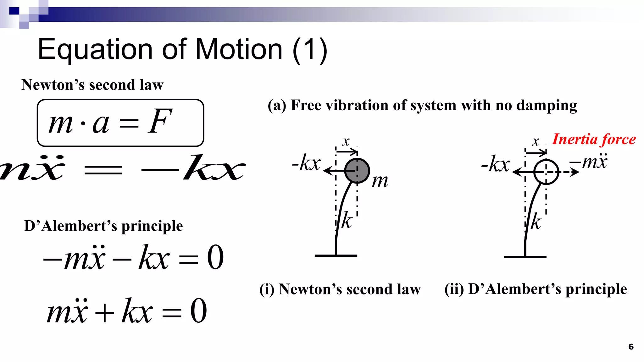
Newton’s second law
m a F
 
mx kx
 
D’Alembert’s principle
0
mx kx
  
0
mx kx
 
x
m
k
-kx
(a) Free vibration of system with no damping
(i) Newton’s second law (ii) D’Alembert’s principle
x
k
-kx mx

Inertia force

7. Equation of Motion (2)
7
x
m
k
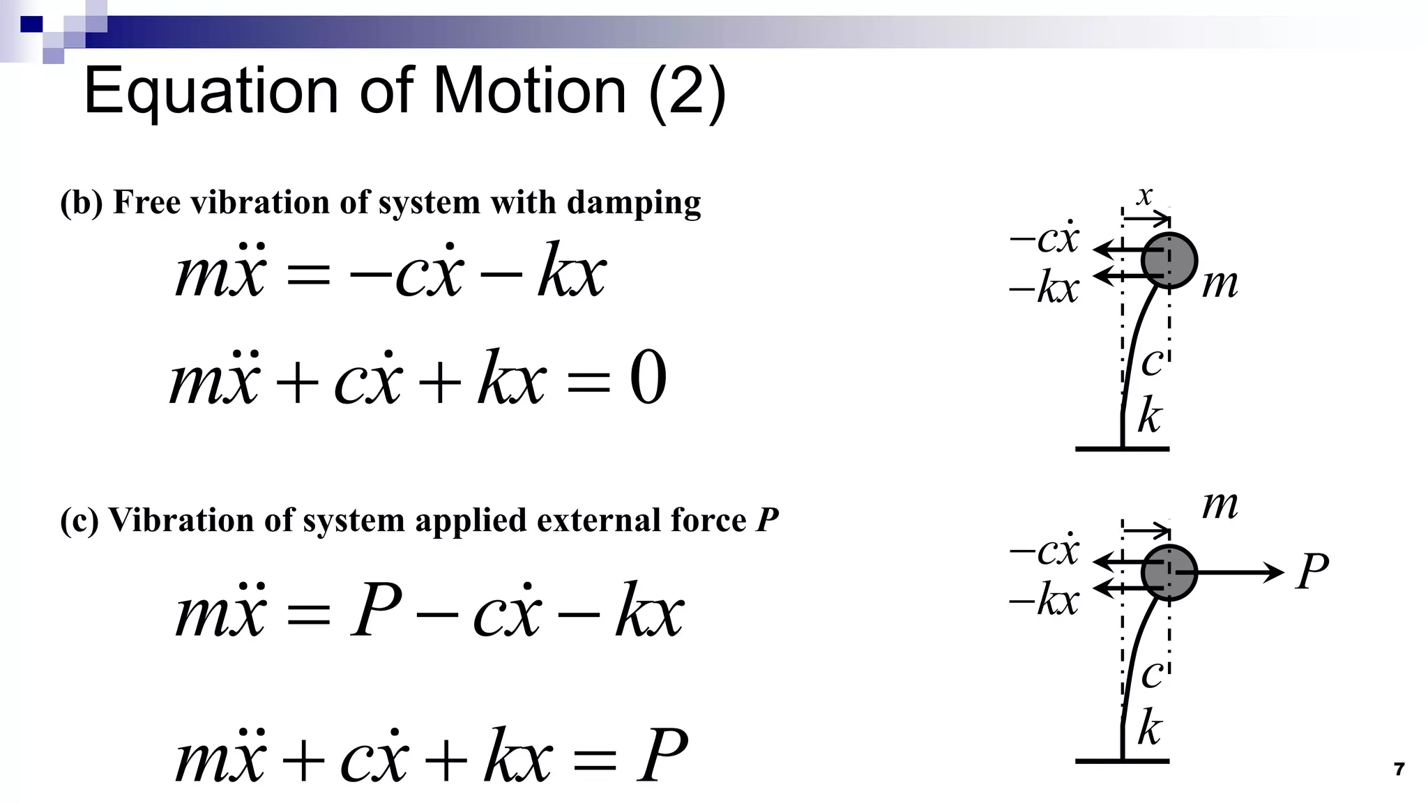
(b) Free vibration of system with damping
(c) Vibration of system applied external force P
mx cx kx
  
0
mx cx kx
   c
cx

kx

m
k
c
cx

kx

P
mx P cx kx
  
mx cx kx P
  

8. Equation of Motion (3)
8
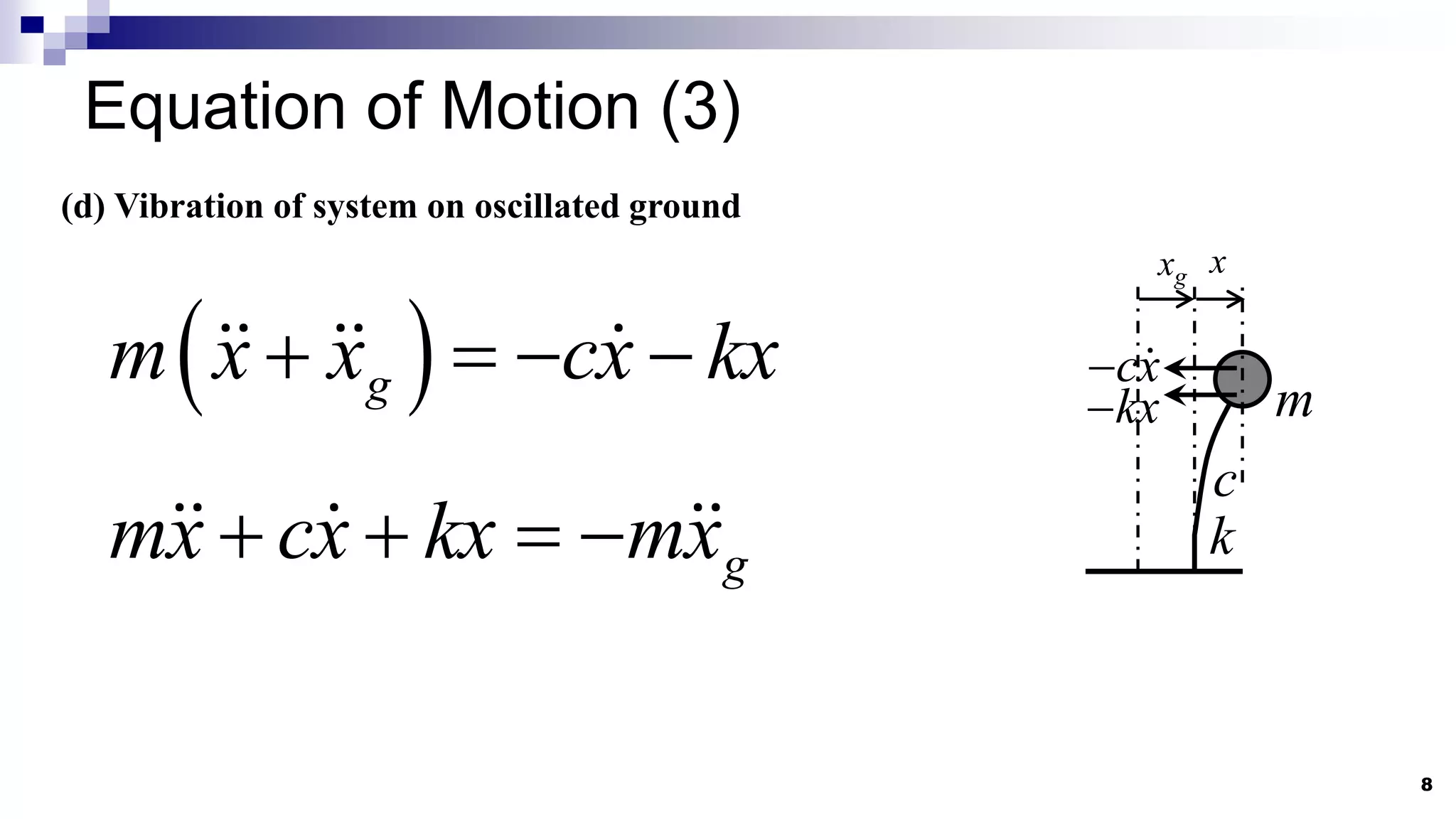
(d) Vibration of system on oscillated ground
 
g
m x x cx kx
   
x
m
k
c
cx

kx

xg
g
mx cx kx mx
   

9. 9
Free Vibration

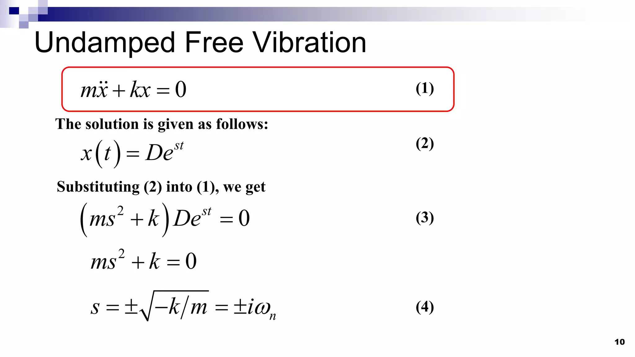
10. Undamped Free Vibration
10
0
mx kx
  (1)
The solution is given as follows:
  st
x t De

(2)
Substituting (2) into (1), we get
 
2
0
st
ms k De
 
2
0
ms k
 
(3)
n
s k m i
     (4)

11. 11
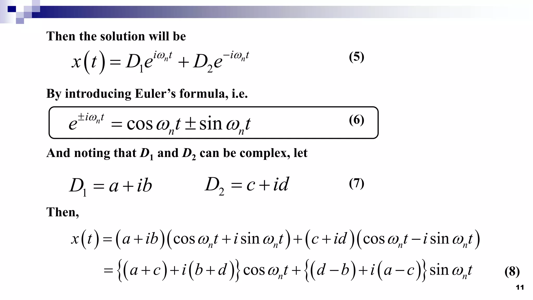
Then the solution will be
  1 2
n n
i t i t
x t D e D e
 

  (5)
cos sin
n
i t
n n
e t t

 

 
By introducing Euler’s formula, i.e.
(6)
And noting that D1 and D2 can be complex, let
1
D a ib
  2
D c id
 
Then,
       
cos sin cos sin
n n n n
x t a ib t i t c id t i t
   
     
(7)
   
     
 
cos sin
n n
a c i b d t d b i a c t
 
        (8)

12. 12
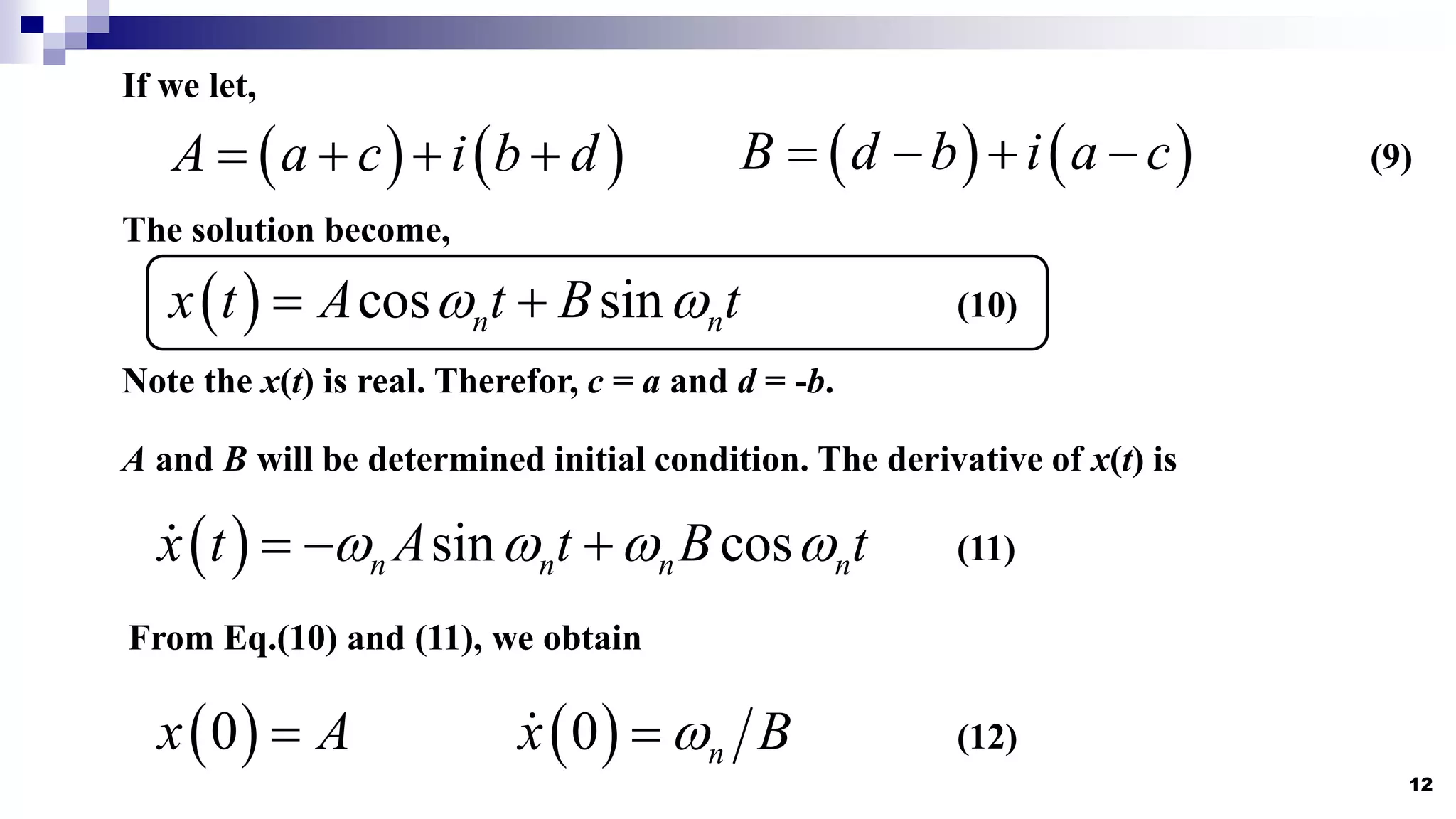
If we let,
   
A a c i b d
       
B d b i a c
   
The solution become,
  cos sin
n n
x t A t B t
 
 
Note the x(t) is real. Therefor, c = a and d = -b.
A and B will be determined initial condition. The derivative of x(t) is
  sin cos
n n n n
x t A t B t
   
  
(9)
(10)
(11)
From Eq.(10) and (11), we obtain
 
0
x A
  
0 n
x B

 (12)

13. 13
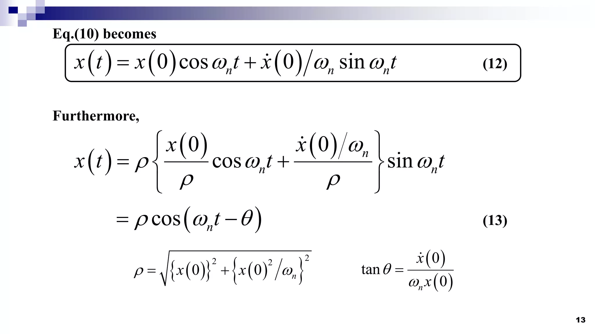
Eq.(10) becomes
     
0 cos 0 sin
n n n
x t x t x t
  
  (12)
Furthermore,
 
   
0 0
cos sin
n
n n
x x
x t t t

  
 
 
 
 
 
 
cos nt
  
  (13)
 
   
 
2
2 2
0 0 n
x x
 
 
 
 
0
tan
0
n
x
x




14. Damped Free Vibration
14
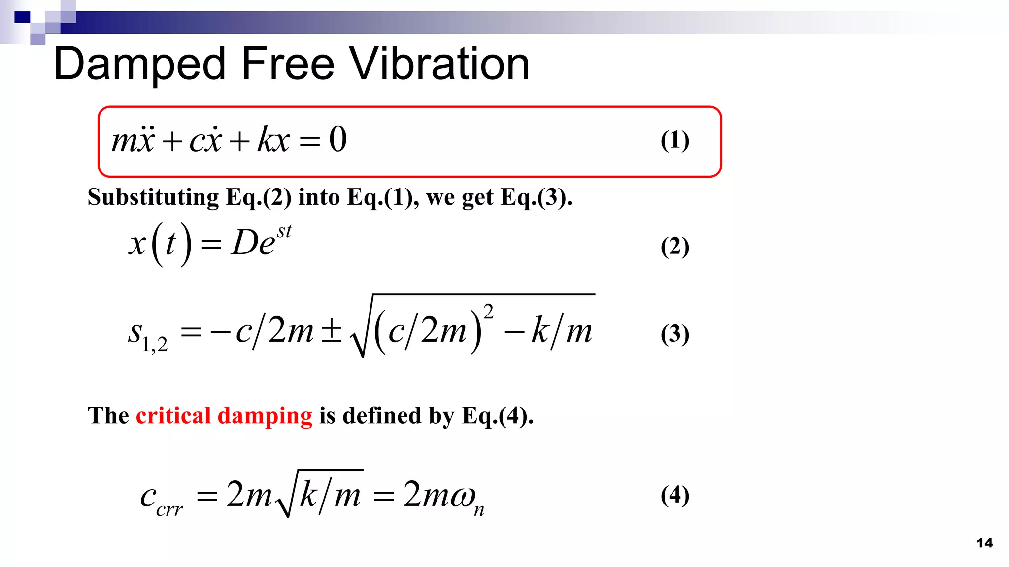
0
mx cx kx
   (1)
  st
x t De

Substituting Eq.(2) into Eq.(1), we get Eq.(3).
 
2
1,2 2 2
s c m c m k m
    (3)
(2)
The critical damping is defined by Eq.(4).
2 2
crr n
c m k m m
  (4)

15. 15
Damped systems are classified into three types.
(a) c<ccrr: Underdamped system
(b) c=ccrr: Critically damped system
(c) c>ccrr: Overdamped system

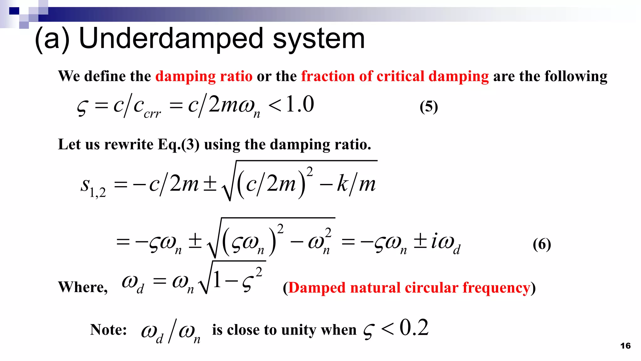
16. (a) Underdamped system
16
We define the damping ratio or the fraction of critical damping are the following
2 1.0
crr n
c c c m
 
   (5)
Let us rewrite Eq.(3) using the damping ratio.
 
2
1,2 2 2
s c m c m k m
   
 
2 2
n n n n d
i
    
       (6)
Where,
2
1
d n
  
  (Damped natural circular frequency)
Note: 0.2
 
d n
  is close to unity when

17. 17
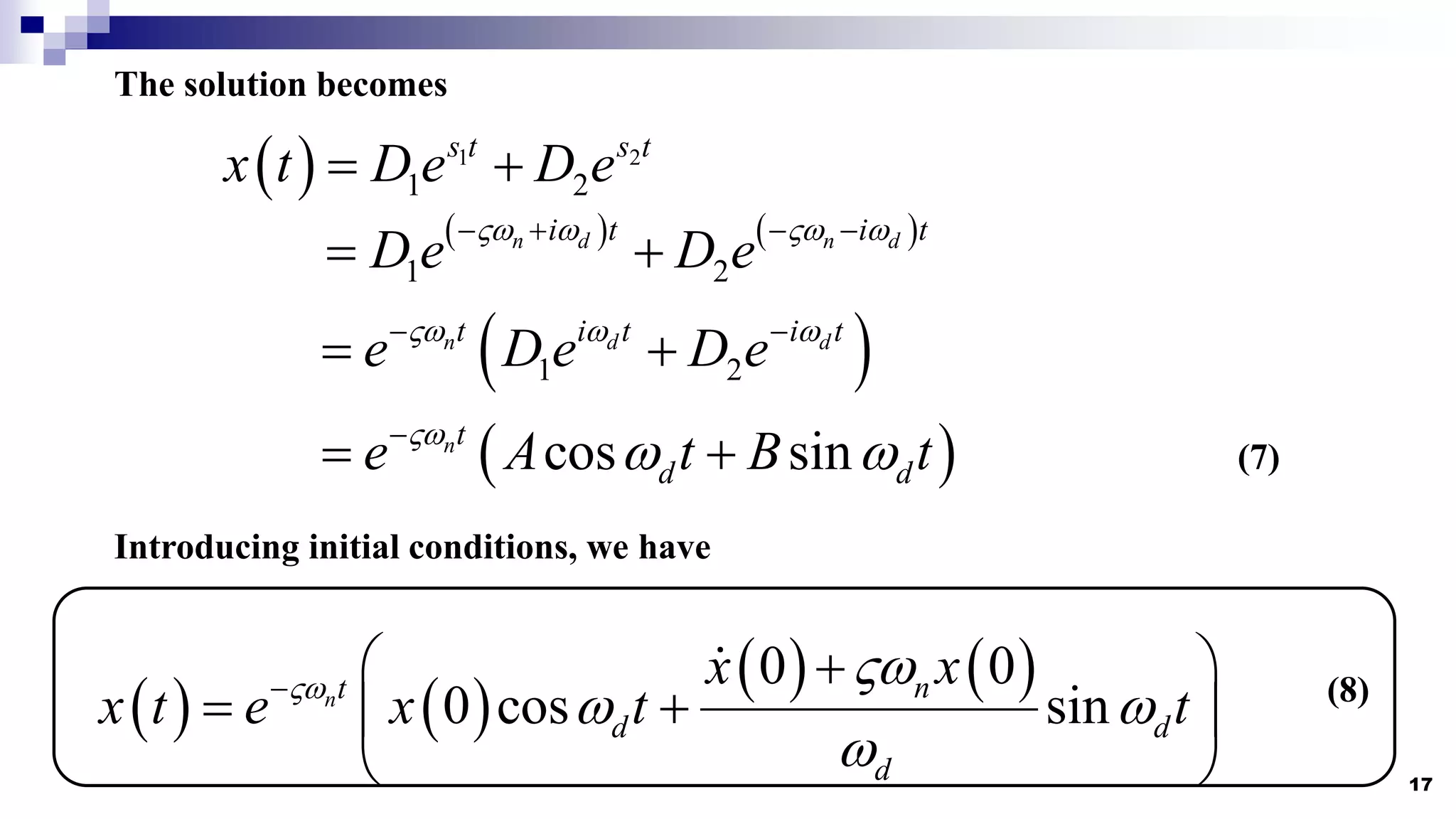
The solution becomes
  1 2
1 2
s t s t
x t D e D e
 
   
1 2
n d n d
i t i t
D e D e
   
   
 
 
1 2
n d d
t i t i t
e D e D e
  
 
 
 
cos sin
nt
d d
e A t B t

 

 
Introducing initial conditions, we have
   
   
0 0
0 cos sin
n n
t
d d
d
x x
x t e x t t
 
 

  

 
 
 
(7)
(8)

18. 18
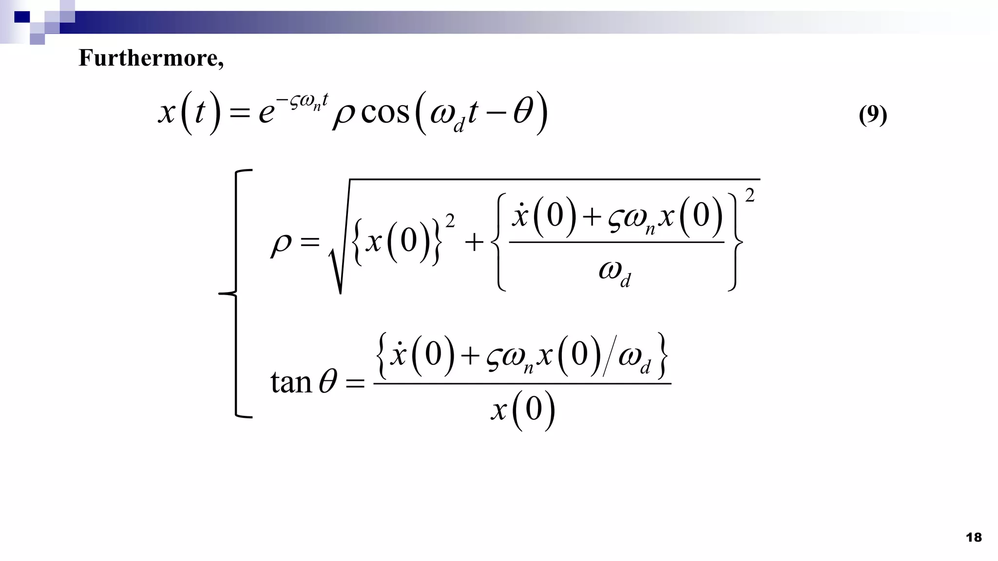
Furthermore,
   
cos
nt
d
x t e t

  

 
 
 
   
2
2 0 0
0 n
d
x x
x



 

   
 
   
 
 
0 0
tan
0
n d
x x
x
 



(9)

19. 19
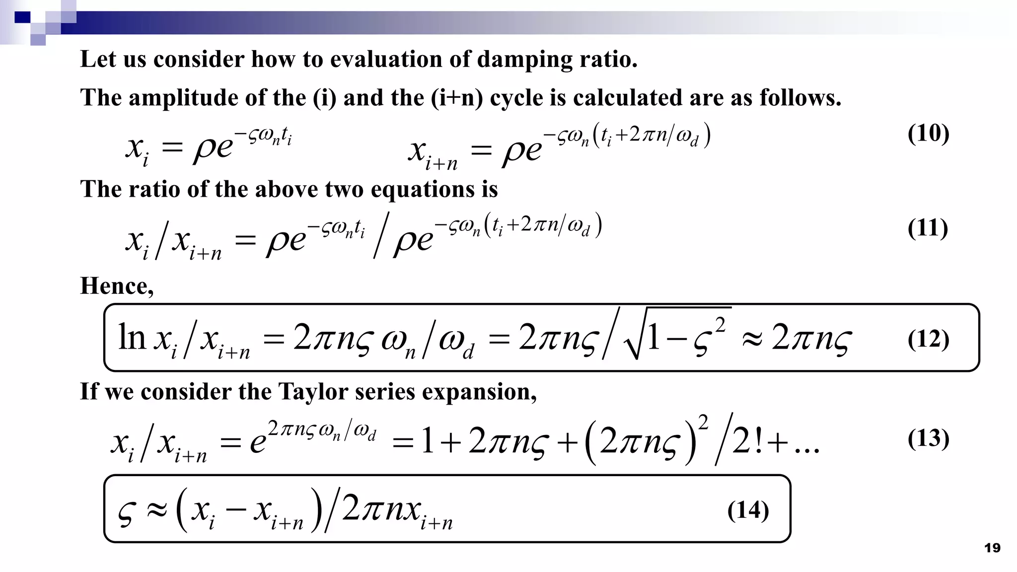
Let us consider how to evaluation of damping ratio.
The amplitude of the (i) and the (i+n) cycle is calculated are as follows.
n i
t
i
x e 
 
  
2
n i d
t n
i n
x e
  
  
 
The ratio of the above two equations is
 
2
n i d
n i t n
t
i i n
x x e e
  

   

 
Hence,
2
ln 2 2 1 2
i i n n d
x x n n n
        
    
If we consider the Taylor series expansion,
 
2
2
1 2 2 2! ...
n d
n
i i n
x x e n n
  
   
     
  2
i i n i n
x x nx
 
 
 
(10)
(11)
(12)
(13)
(14)

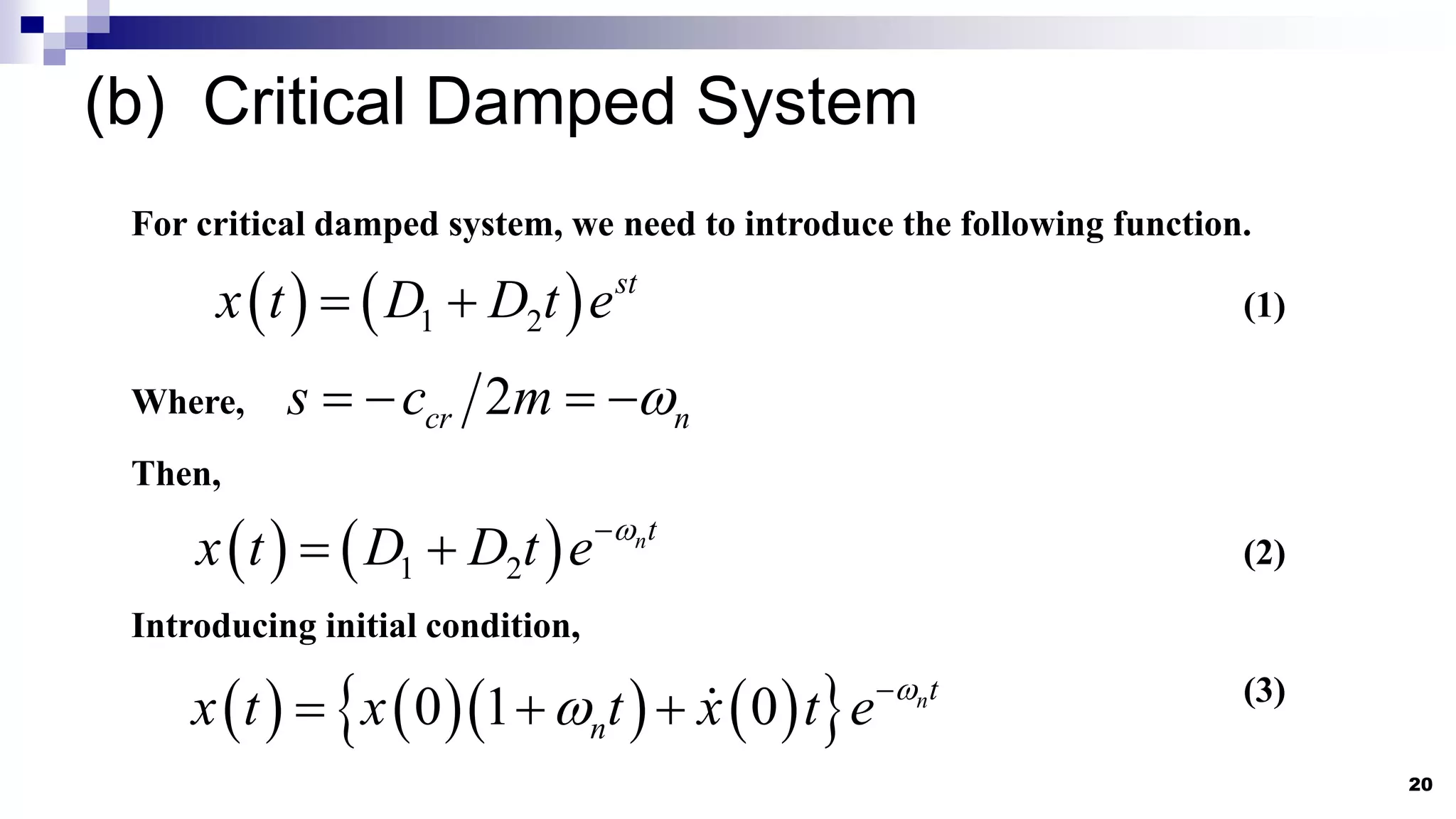
20. (b) Critical Damped System
20
For critical damped system, we need to introduce the following function.
   
1 2
st
x t D D t e
  (1)
Where, 2
cr n
s c m 
   
Then,
   
1 2
nt
x t D D t e 

  (2)
Introducing initial condition,
      
 
0 1 0 nt
n
x t x t x t e 
 
   (3)

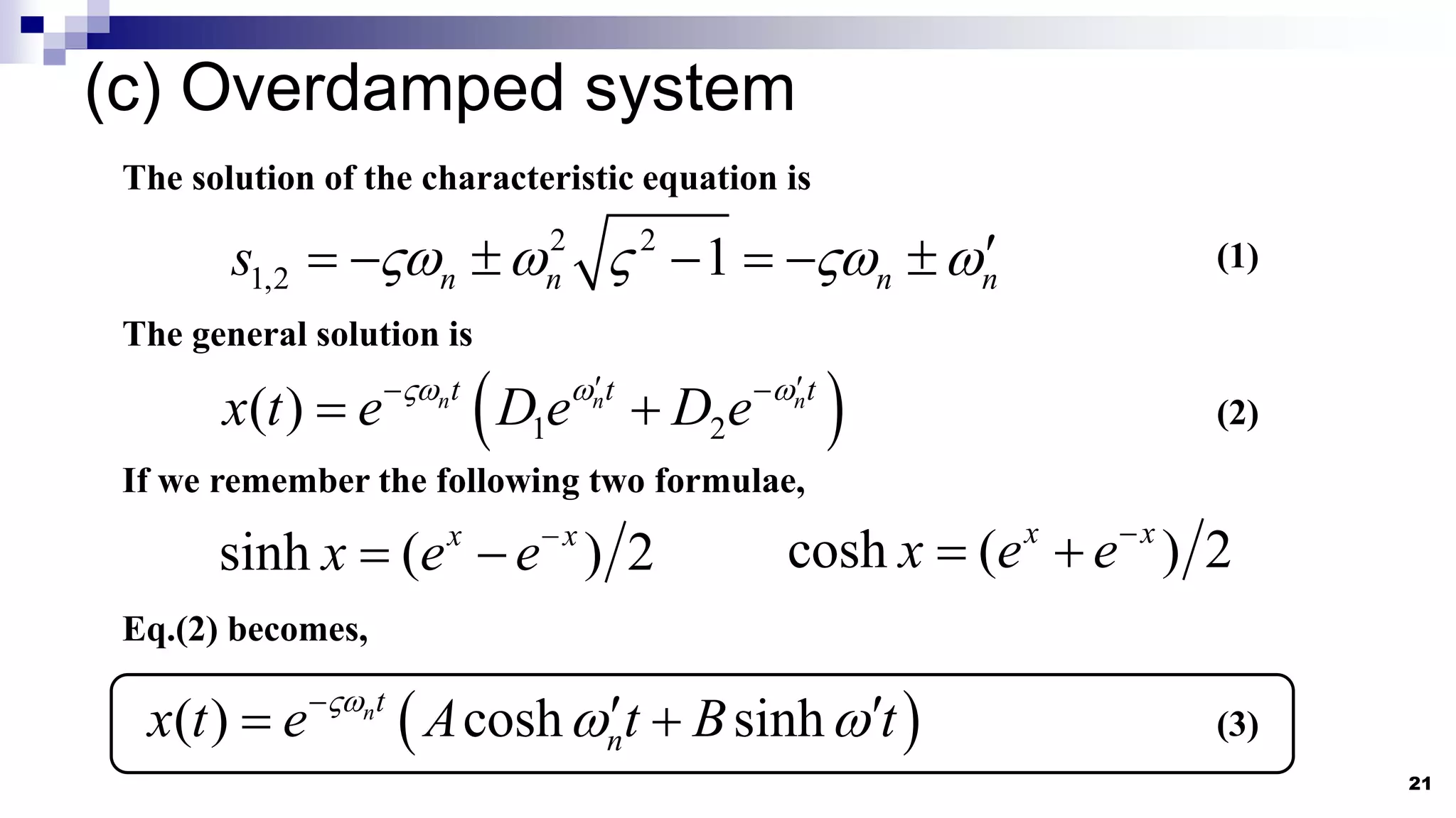
21. (c) Overdamped system
21
2 2
1,2 1
n n n n
s     
      
The solution of the characteristic equation is
(1)
The general solution is
 
1 2
( ) n n n
t t t
x t e D e D e
  
 
 
  (2)
If we remember the following two formulae,
sinh ( ) 2
x x
x e e
  cosh ( ) 2
x x
x e e
 
Eq.(2) becomes,
 
( ) cosh sinh
nt
n
x t e A t B t

 

 
  (3)

22. 22
Response to Harmonic Loading

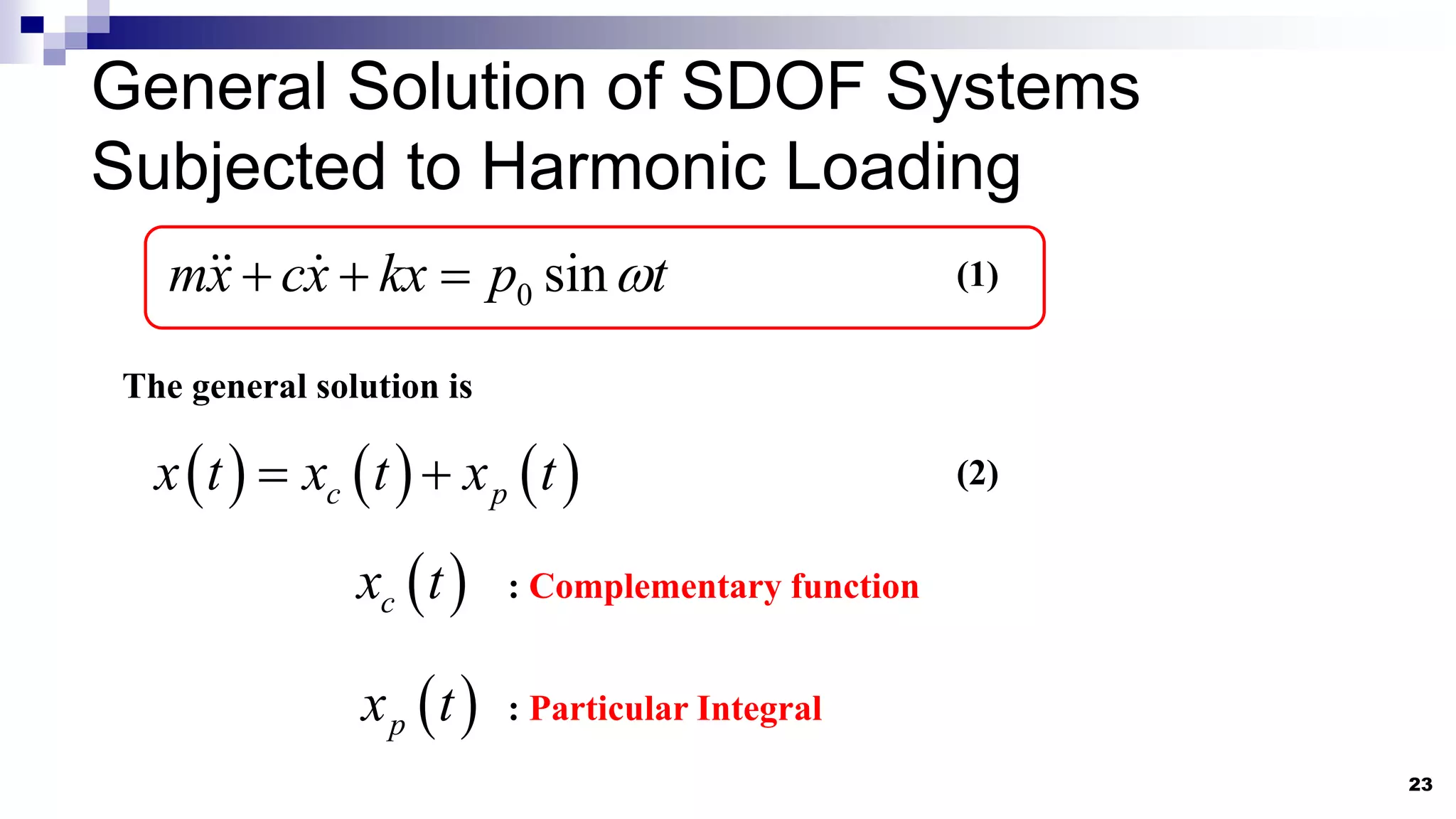
23. General Solution of SDOF Systems
Subjected to Harmonic Loading
23
0 sin
mx cx kx p t

   (1)
The general solution is
     
c p
x t x t x t
 
 
c
x t
 
p
x t
: Complementary function
: Particular Integral
(2)

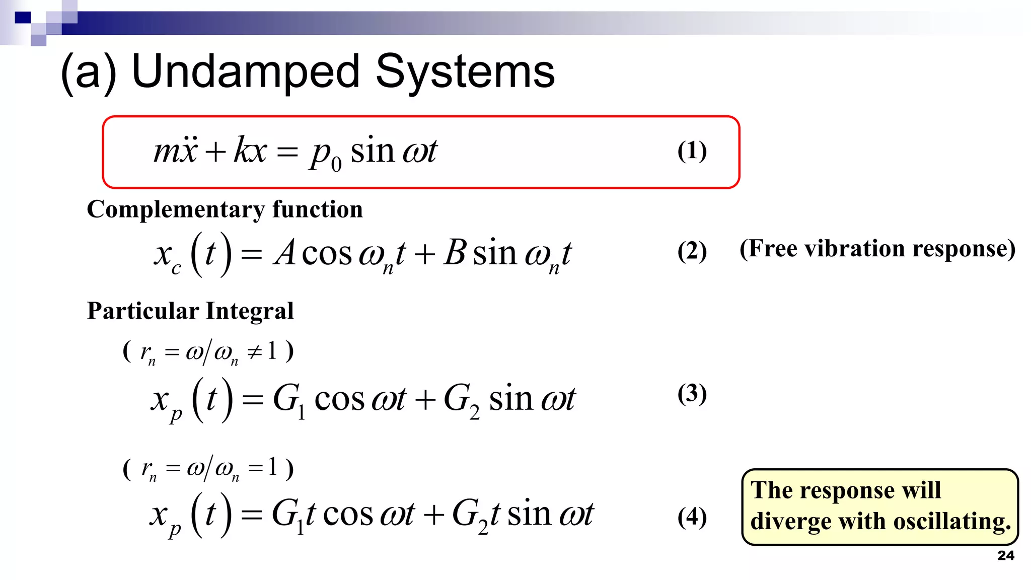
24. (a) Undamped Systems
24
0 sin
mx kx p t

  (1)
Complementary function
  cos sin
c n n
x t A t B t
 
  (Free vibration response)
Particular Integral
  1 2
cos sin
p
x t G t G t
 
 
( )
1
n n
r  
 
( )
1
n n
r  
 
  1 2
cos sin
p
x t G t t G t t
 
 
The response will
diverge with oscillating.
(2)
(3)
(4)

25. 25
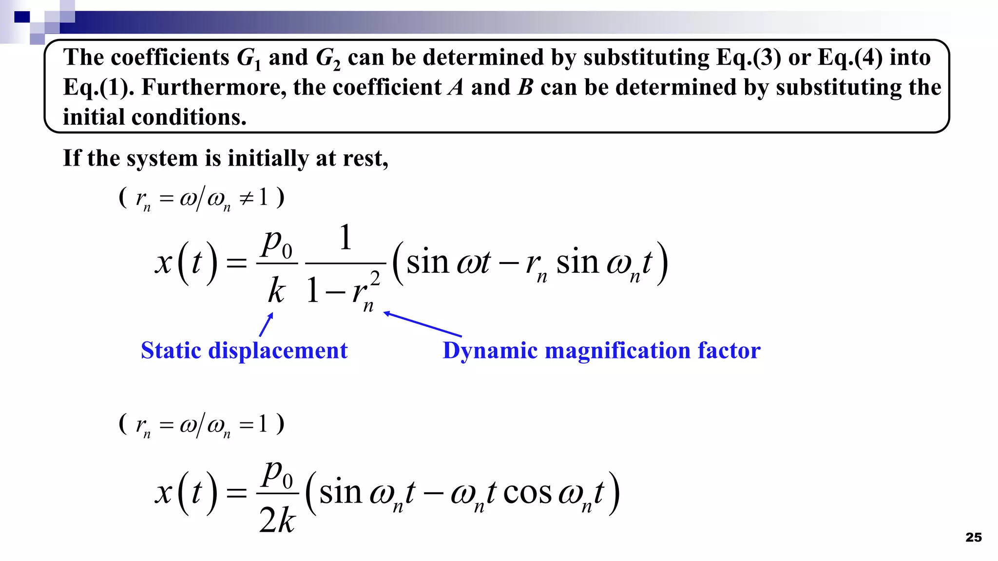
The coefficients G1 and G2 can be determined by substituting Eq.(3) or Eq.(4) into
Eq.(1). Furthermore, the coefficient A and B can be determined by substituting the
initial conditions.
If the system is initially at rest,
( )
1
n n
r  
 
( )
1
n n
r  
 
   
0
2
1
sin sin
1
n n
n
p
x t t r t
k r
 
 

Static displacement Dynamic magnification factor
   
0
sin cos
2
n n n
p
x t t t t
k
  
 

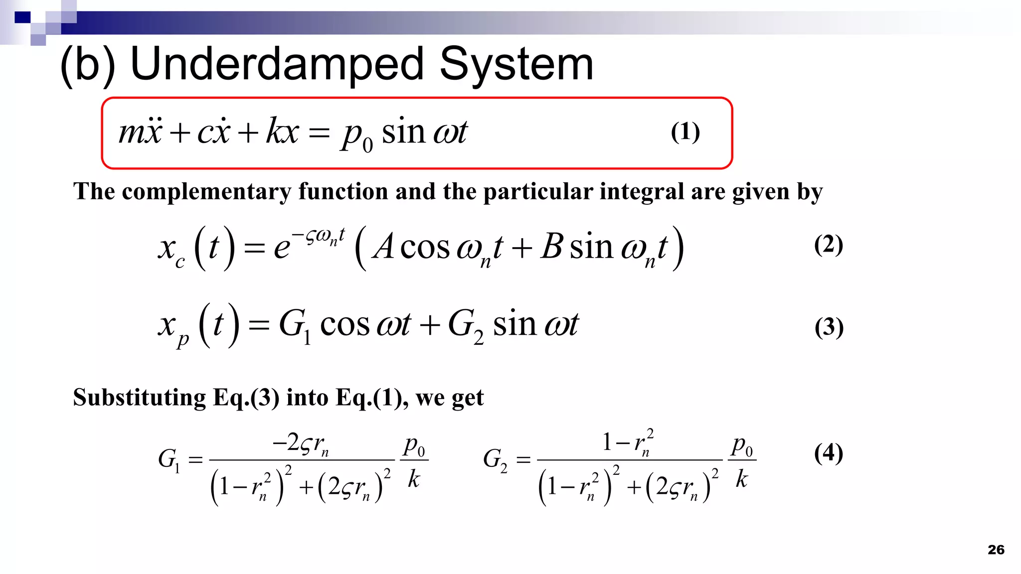
26. (b) Underdamped System
26
0 sin
mx cx kx p t

   (1)
   
cos sin
nt
c n n
x t e A t B t

 

 
  1 2
cos sin
p
x t G t G t
 
 
The complementary function and the particular integral are given by
(2)
(3)
   
0
1 2 2
2
2
1 2
n
n n
r p
G
k
r r




     
2
0
2 2 2
2
1
1 2
n
n n
r p
G
k
r r



 
Substituting Eq.(3) into Eq.(1), we get
(4)

27. 27
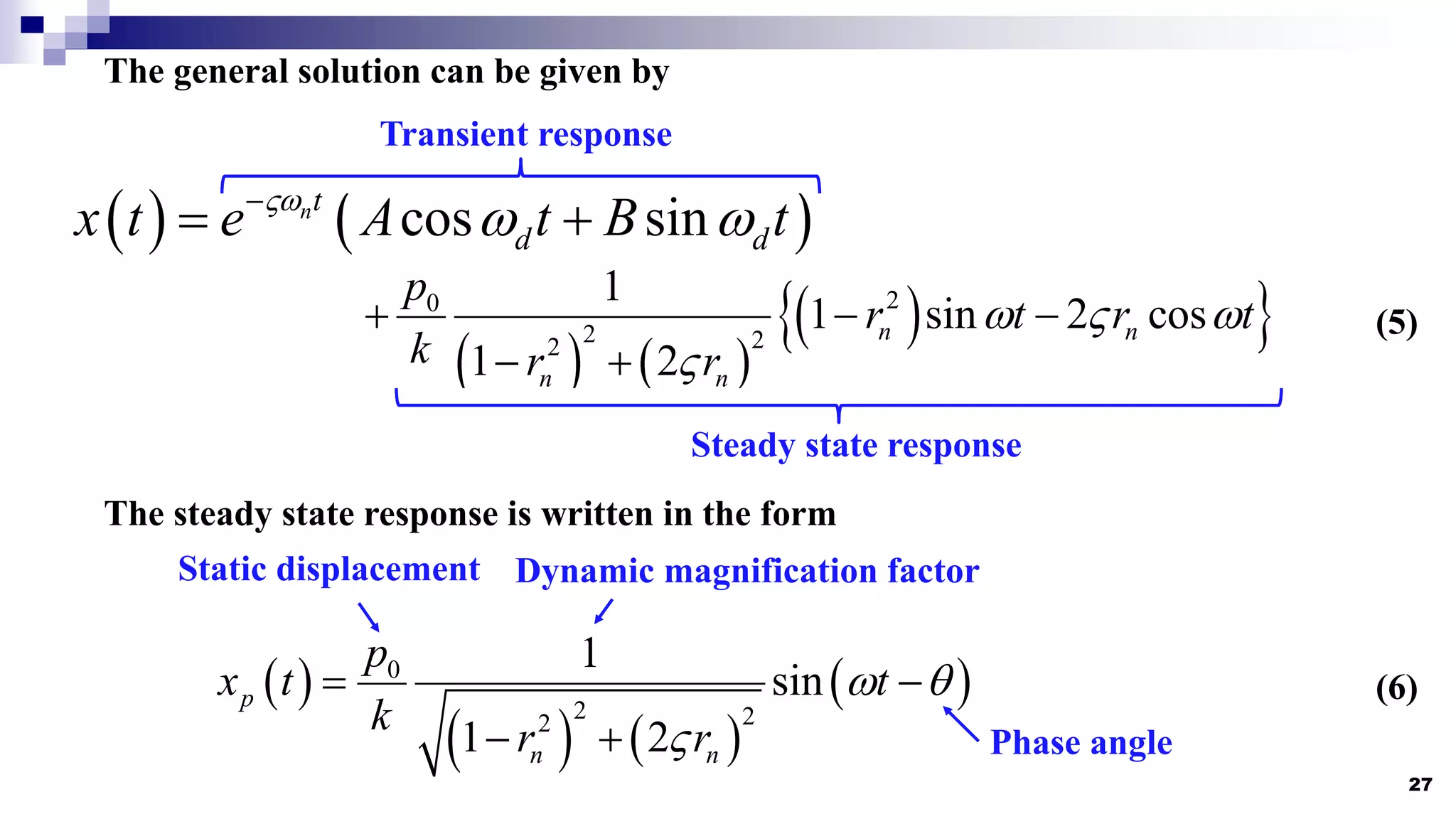
The general solution can be given by
   
cos sin
nt
d d
x t e A t B t

 

 
   
 
 
2
0
2 2
2
1
1 sin 2 cos
1 2
n n
n n
p
r t r t
k r r
  

  
 
Transient response
Steady state response
The steady state response is written in the form
 
   
 
0
2 2
2
1
sin
1 2
p
n n
p
x t t
k r r
 

 
 
Static displacement Dynamic magnification factor
Phase angle
(5)
(6)

28. 28
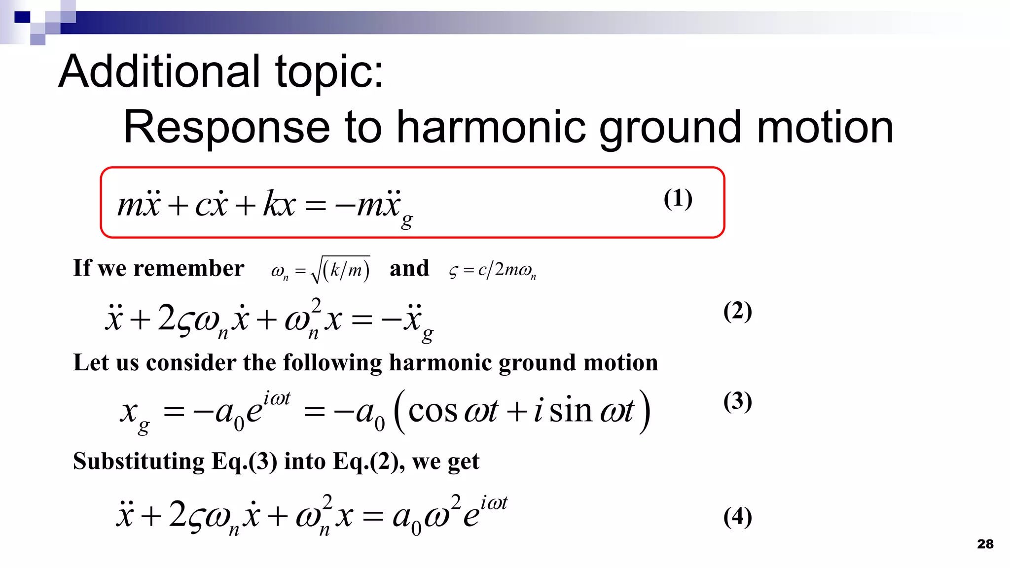
Additional topic:
Response to harmonic ground motion
g
mx cx kx mx
   
2
2 n n g
x x x x
 
   
If we remember and
 
n k m
  2 n
c m
 

Let us consider the following harmonic ground motion
 
0 0 cos sin
i t
g
x a e a t i t

 
    
(1)
(2)
(3)
Substituting Eq.(3) into Eq.(2), we get
2 2
0
2 i t
n n
x x x a e 
  
   (4)

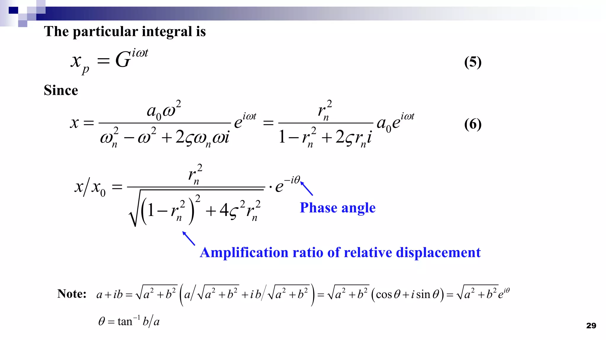
29. 29
The particular integral is
i t
p
x G 
 (5)
Since
2 2
0
0
2 2 2
2 1 2
i t i t
n
n n n n
a r
x e a e
i r r i
 

    
 
   
(6)
 
2
0 2
2 2 2
1 4
i
n
n n
r
x x e
r r



 
 
   
2 2 2 2 2 2 2 2 2 2
cos sin i
a ib a b a a b ib a b a b i a b e
 
          
Note:
1
tan b a
 

Phase angle
Amplification ratio of relative displacement

30. 30
Amplification ratio Phase lag
z=0.0
z=0.1
z=0.2
z=0.4
z=0.707
z=1.0
z=0.0
z=1.0
z=0.1
z=0.2
z=0.707
z=0.4

31. 31
Phase angle
1
2
2
tan
1
n
n
r
r

 


0
n
r  0.5
n
r  0.8
n
r  1.2
n
r  2.0
n
r  n
r  
0
   

0.99
 

0.84
 

0.13
 

0.02
 

0.1
 

32. 32
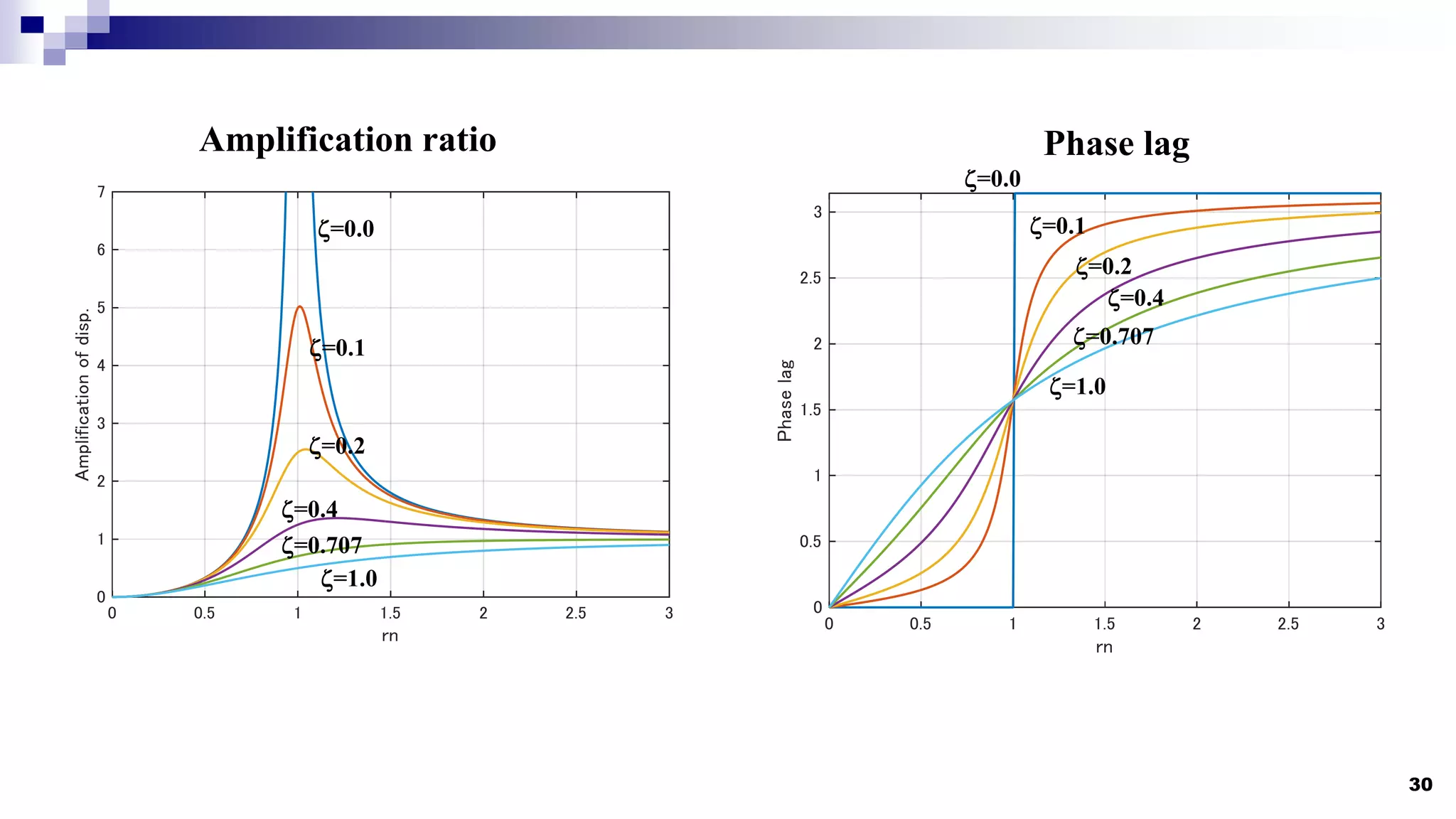
Tool for drawing a graph
rn=0.0:0.01:3.0;
h=[0.0, 0.1, 0.2, 0.4, 0.707, 1.0];
y_y0=zeros(length(rn),length(h));
for ii=1:1:length(h)
for jj=1:1:length(rn)
y_y0(jj,ii)=rn(jj)^2/sqrt((1-rn(jj)^2)^2 + 4*h(ii)^2*rn(jj)^2);
end
end
plot(rn, y_y0, 'linewidth',1.5)
grid on
xlabel('rn')
ylabel('Amplification of disp.')
ylim([0,7])
Definition of
resonance curve
Set of variable
Drawing a graph
Script of MATLAB

33. 33
Response to Arbitrary Loading

34. Methodologies
34
(2) Duhamel Integral
(1) Response history analysis
(3) Frequency domain analysis

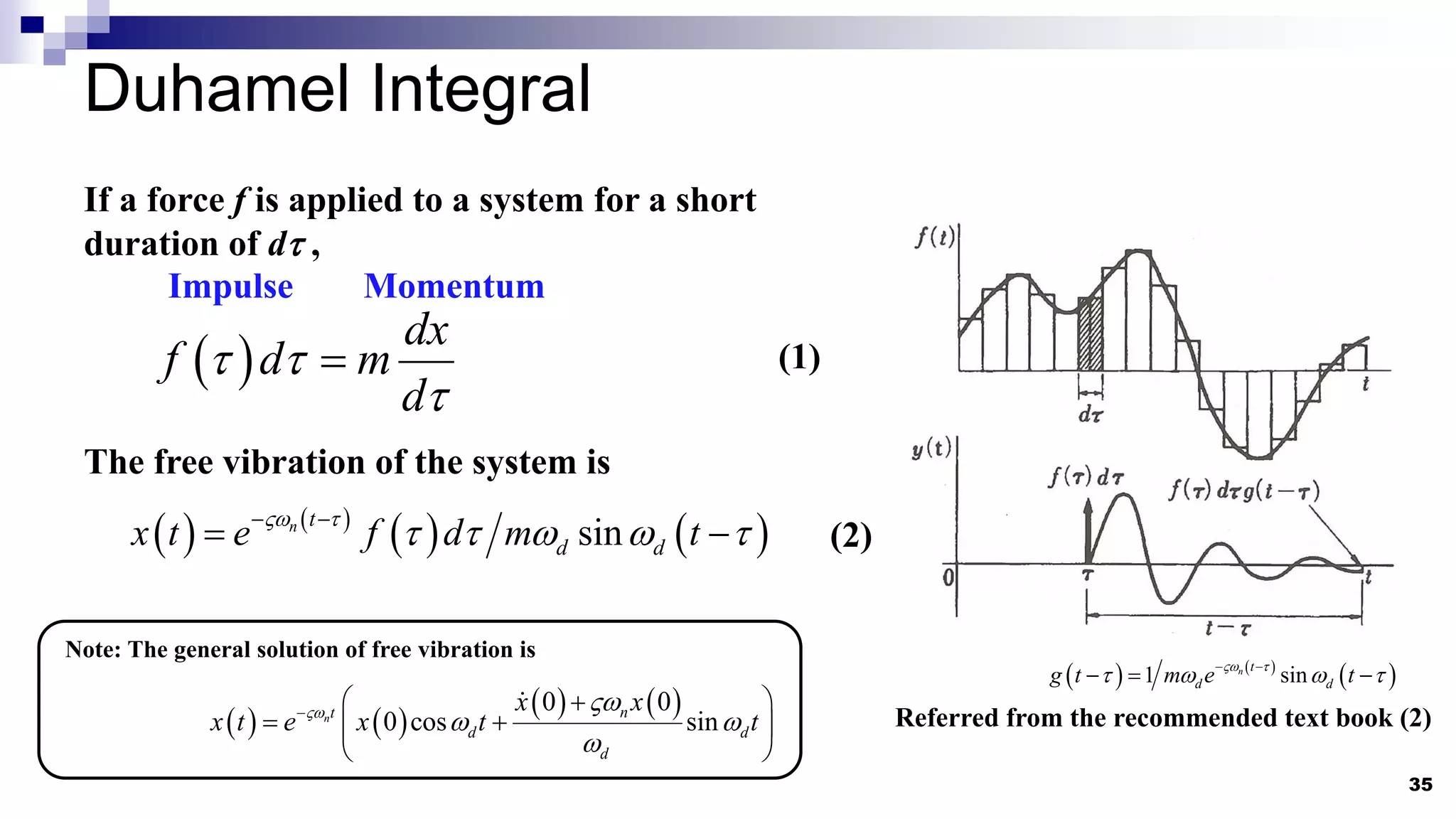
35. Duhamel Integral
35
Referred from the recommended text book (2)
If a force f is applied to a system for a short
duration of dt ,
 
dx
f d m
d
t t
t

Impulse Momentum
   
   
sin
n t
d d
x t e f d m t
 t
t t   t
 
 
The free vibration of the system is
Note: The general solution of free vibration is
   
   
0 0
0 cos sin
n n
t
d d
d
x x
x t e x t t
 
 

  

 
 
 
   
 
1 sin
n t
d d
g t m e t
 t
t   t
 
  
(1)
(2)

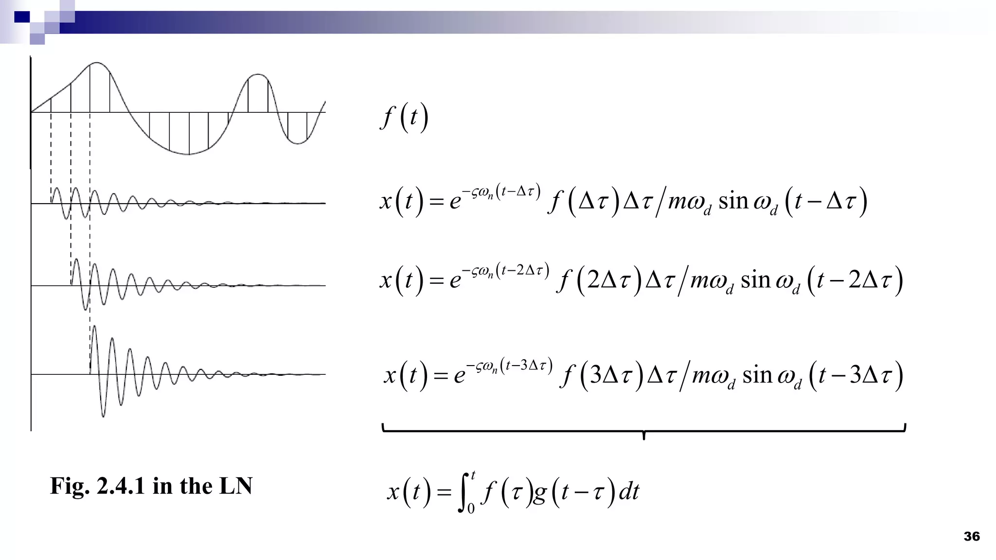
36. 36
Fig. 2.4.1 in the LN
   
   
sin
n t
d d
x t e f m t
 t
t t   t
 
    
   
   
2
2 sin 2
n t
d d
x t e f m t
 t
t t   t
  
    
   
   
3
3 sin 3
n t
d d
x t e f m t
 t
t t   t
  
    
 
f t
     
0
t
x t f g t dt
t t
 


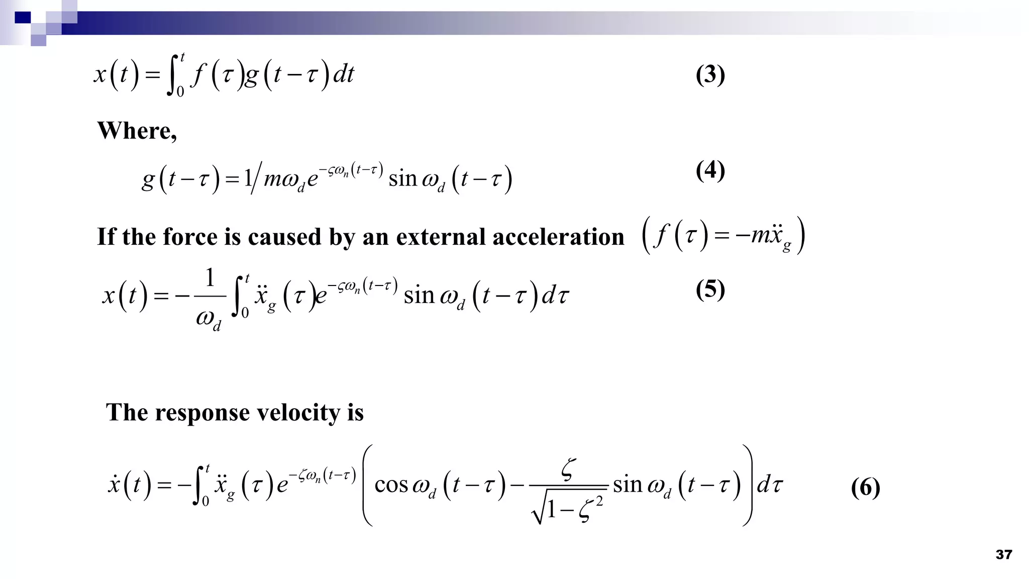
37. 37
     
0
t
x t f g t dt
t t
 

   
 
1 sin
n t
d d
g t m e t
 t
t   t
 
  
Where,
(3)
(4)
If the force is caused by an external acceleration  
 
g
f mx
t  
     
 
0
1
sin
n
t t
g d
d
x t x e t d
 t
t  t t

 
  

The response velocity is
     
   
2
0
cos sin
1
n
t t
g d d
x t x e t t d
z t z
t  t  t t
z
 
 
 
    
 

 
 (6)
(5)

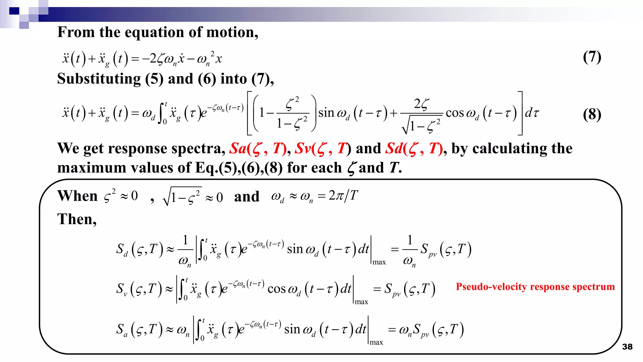
38. 38
From the equation of motion,
    2
2
g n n
x t x t x x
z 
    (7)
Substituting (5) and (6) into (7),
       
   
2
2 2
0
2
1 sin cos
1 1
n
t t
g d g d d
x t x t x e t t d
z t z z
 t  t  t t
z z
 
 
 
     
 
 
 
 
 
 
 (8)
We get response spectra, Sa(z , T), Sv(z , T) and Sd(z , T), by calculating the
maximum values of Eq.(5),(6),(8) for each z and T.
When ,
2
0
  2
1 0

  and 2
d n T
  
 
Then,
     
   
0 max
1 1
, sin ,
n
t t
d g d pv
n n
S T x e t dt S T
z t
 t  t 
 
 
  

     
   
0 max
, cos ,
n
t t
v g d pv
S T x e t dt S T
z t
 t  t 
 
  

     
   
0 max
, sin ,
n
t t
a n g d n pv
S T x e t dt S T
z t
  t  t  
 
  

Pseudo-velocity response spectrum

39. 39
Fig. 2.4.4 Typical characteristics of response spectra
1
n


n



40. 40
Multi Degree Freedom Systems
(Modal response analysis)

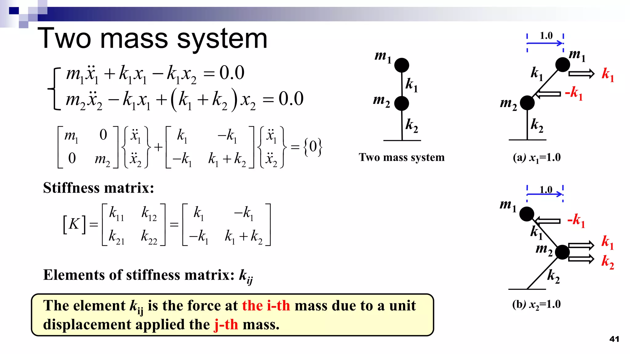
41. Two mass system
41
1.0
m1
m2
k1
k2
k1
-k1
1.0
m2
m1
k1
k2
-k1
k1
k2
1 1 1 1 1 2 0.0
m x k x k x
  
 
2 2 1 1 1 2 2 0.0
m x k x k k x
   
 
1 1 1 1 1
2 2 1 1 2 2
0
0
0
m x k k x
m x k k k x

       
 
   
   
 
       
Stiffness matrix:
m2
m1
k2
k1
Two mass system (a) x1=1.0
(b) x2=1.0
  11 12 1 1
21 22 1 1 2
k k k k
K
k k k k k

   
 
   
 
   
Elements of stiffness matrix: kij
The element kij is the force at the i-th mass due to a unit
displacement applied the j-th mass.

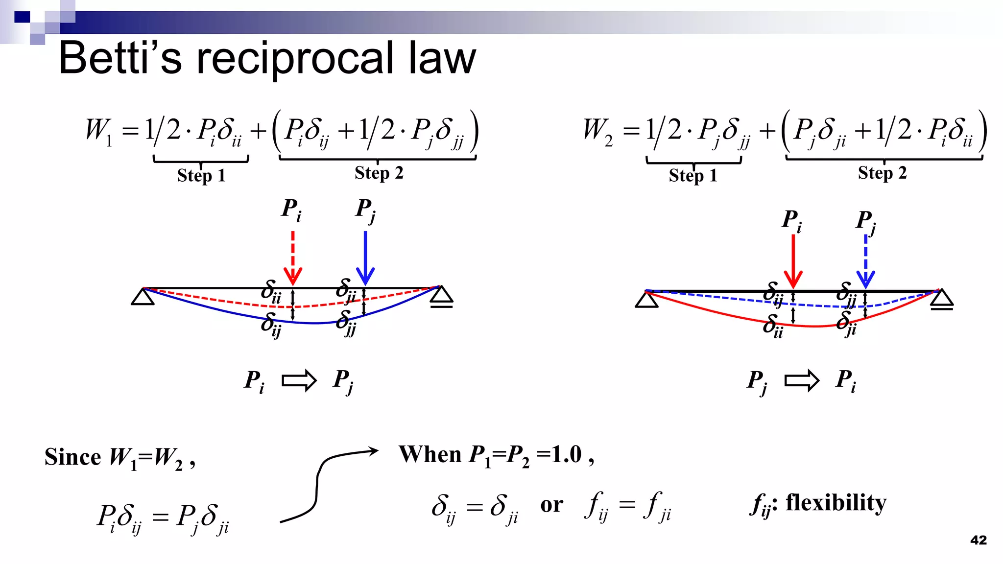
42. Betti’s reciprocal law
42
 
1 1 2 1 2
i ii i ij j jj
W P P P
  
      
2 1 2 1 2
j jj j ji i ii
W P P P
  
    
Pi Pj
ii
ij
ji
jj
Pi Pj
ij
ii
jj
ji
Pi Pj Pj Pi
Since W1=W2 ,
Step 1 Step 2 Step 2
Step 1
i ij j ji
P P
 

When P1=P2 =1.0 ,
ij ji
 
 or ij ji
f f
 fij: flexibility

43. 43
   
1
K F


The stiffness matrix [K] is symmetry as well as the flexible matrix [F].
Example of stiffness matrix;
1
n
i
i-1
i+1
1 1
1 1
1 1
1 1
0
0
i i i i
i i i i
n n n
k k
k k k k
k k k k
k k k
 
 
 

  
  
 
i
i
Symmetric and Sparse

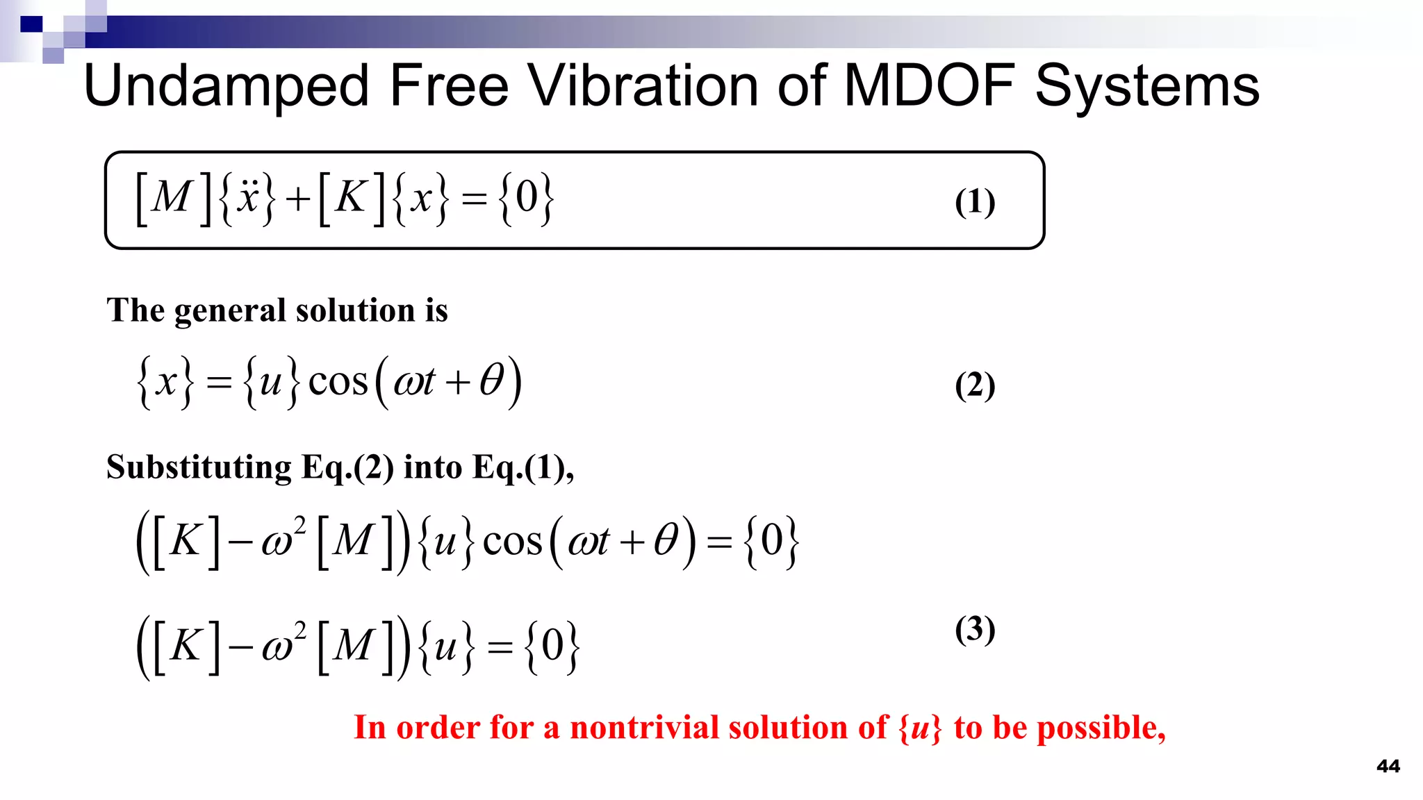
44. Undamped Free Vibration of MDOF Systems
44
       
0
M x K x
 
The general solution is
     
cos
x u t
 
 
(1)
(2)
Substituting Eq.(2) into Eq.(1),
   
      
2
cos 0
K M u t
  
  
   
    
2
0
K M u

  (3)
In order for a nontrivial solution of {u} to be possible,

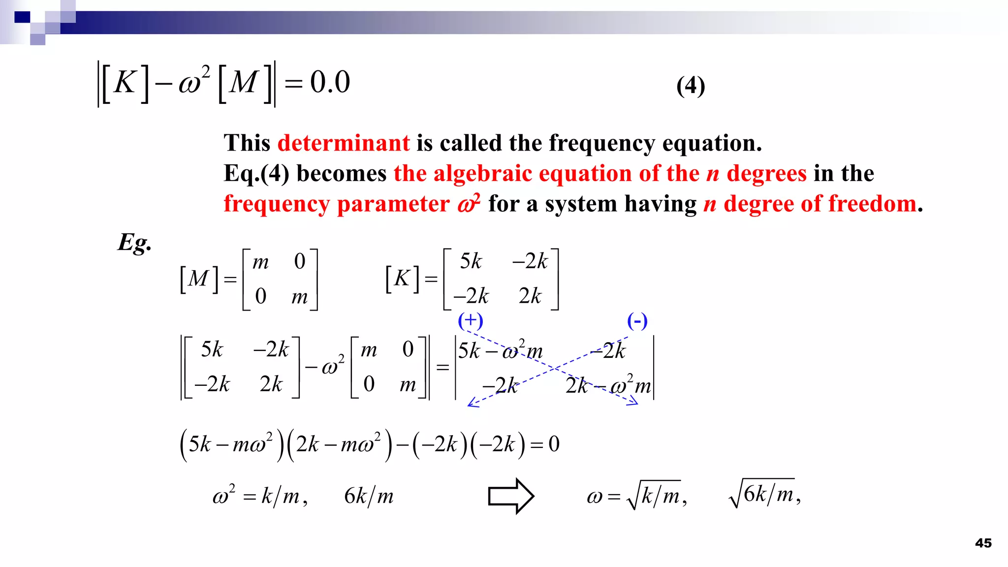
45. 45
   
2
0.0
K M

  (4)
This determinant is called the frequency equation.
Eq.(4) becomes the algebraic equation of the n degrees in the
frequency parameter 2 for a system having n degree of freedom.
 
0
0
m
M
m
 
  
 
 
5 2
2 2
k k
K
k k

 
  

 
Eg.
2
2
2
5 2 0 5 2
2 2 0 2 2
k k m k m k
k k m k k m



  
   
 
   
  
   
     
2 2
5 2 2 2 0
k m k m k k
 
     
2
,
k m
  6k m ,
k m
  6 ,
k m
(-)
(+)

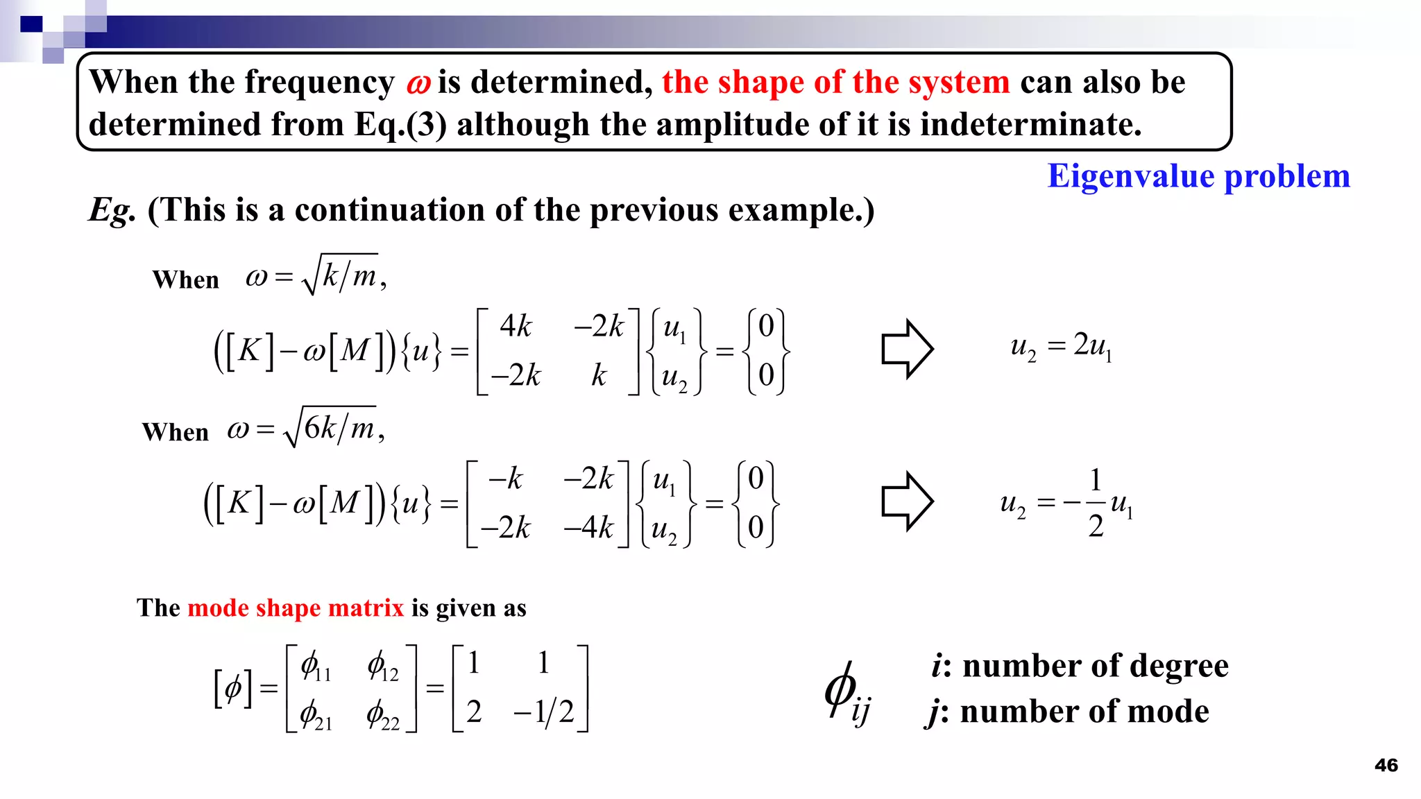
46. 46
When the frequency  is determined, the shape of the system can also be
determined from Eq.(3) although the amplitude of it is indeterminate.
Eg. (This is a continuation of the previous example.)
,
k m
 
When
   
   1
2
4 2 0
2 0
u
k k
K M u
u
k k

  
   
  
   
 

   
 
2 1
2
u u

6 ,
k m
 
When
   
   1
2
2 0
2 4 0
u
k k
K M u
u
k k

   
   
  
   
 
 
   
 
2 1
1
2
u u
 
The mode shape matrix is given as
  11 12
21 22
1 1
2 1 2
 

 
   
 
   

 
 
Eigenvalue problem
ij
 i: number of degree
j: number of mode

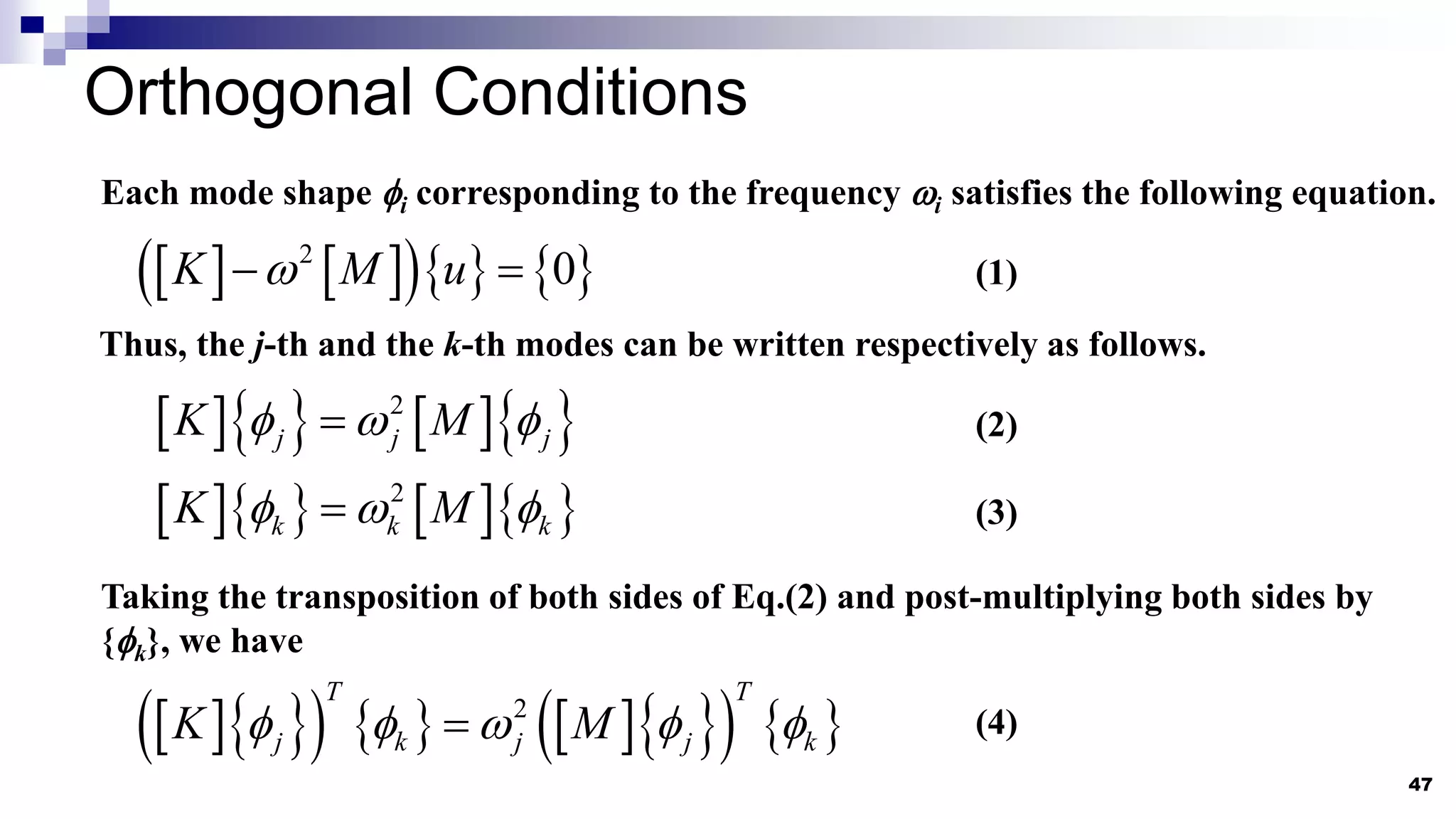
47. Orthogonal Conditions
47
   
    
2
0
K M u

 
Each mode shape i corresponding to the frequency i satisfies the following equation.
Thus, the j-th and the k-th modes can be written respectively as follows.
     
2
j j j
K M
  

     
2
k k k
K M
  

Taking the transposition of both sides of Eq.(2) and post-multiplying both sides by
{k}, we have
(1)
(2)
(3)
  
      
   
2
T T
j k j j k
K M
    
 (4)

48. 48
Remembering the relation ([A][B])T=[B] T[A] T, and the matrices [K] and [M] are
symmetrical, i.e. [K] T =[K] and [M] T =[M], Eq.(4) becomes
         
2
T T
j k j j k
K M
    
 (5)
Pre-multiplying both sides of Eq.(3) by {j}T, we have
         
2
T T
j k k j k
K M
    
 (6)
Eq.(6) is subtracted from each side of Eq.(5).
     
2 2
0
T
j k j k
M
   
  (7)
Apparently, . We have for different mode shapes
2 2
j k
 

     0
T
j k
M
   (8)
for
2 2
j k
 

First orthogonality of
eigenvectors

49. 49
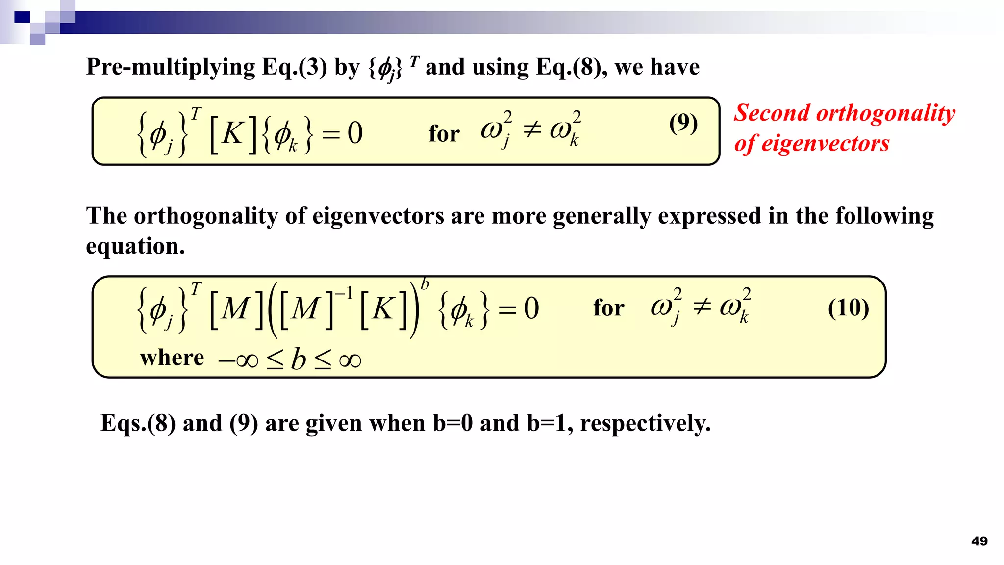
Pre-multiplying Eq.(3) by {j} T and using Eq.(8), we have
     0
T
j k
K
   (9)
for
2 2
j k
 

Second orthogonality
of eigenvectors
The orthogonality of eigenvectors are more generally expressed in the following
equation.
       
   
1
0
b
T
j k
M M K
 

 (10)
for
2 2
j k
 

where b
   
Eqs.(8) and (9) are given when b=0 and b=1, respectively.

50. 50
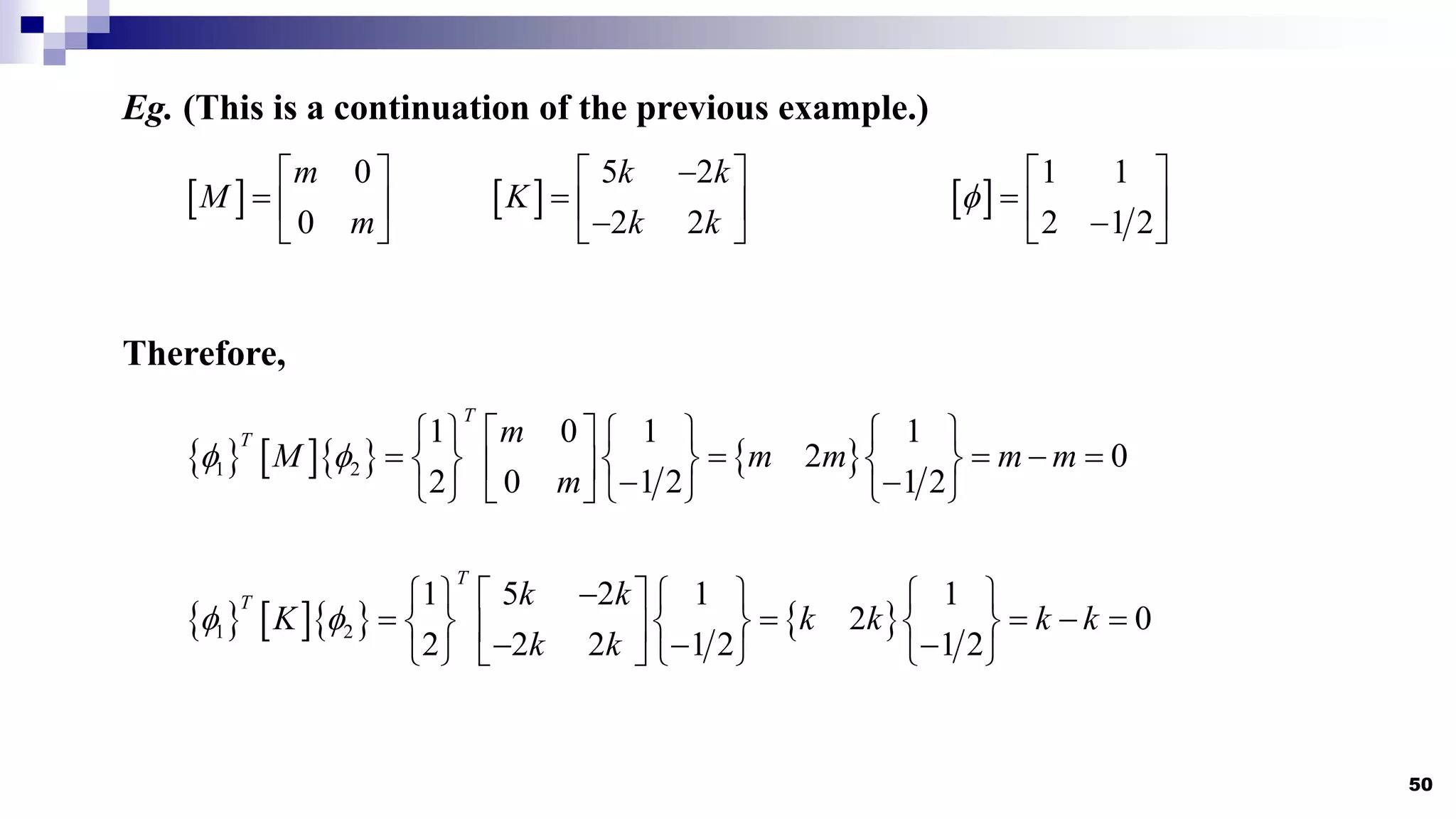
Eg. (This is a continuation of the previous example.)
 
5 2
2 2
k k
K
k k

 
  

 
 
0
0
m
M
m
 
  
 
 
1 1
2 1 2

 
  

 
Therefore,
      
1 2
1 0 1 1
2 0
2 0 1 2 1 2
T
T m
M m m m m
m
 
       
    
     
   
       
      
1 2
1 5 2 1 1
2 0
2 2 2 1 2 1 2
T
T k k
K k k k k
k k
 

       
    
     
 
  
       

51. Concept of Normal Coordinates
51
Coordinate transformation with mode shape matrix []:
            
1 1 2 2 n n i i
x q q q q q
    
    

Remembering orthogonality of the eigen vectors,
    
    
T
i
i T
i i
M x
q
M

 
 1
i n

Fig. 3.4.1 Concept of Normal Coordinates
q1× q2× q3×
(1)

52. 52
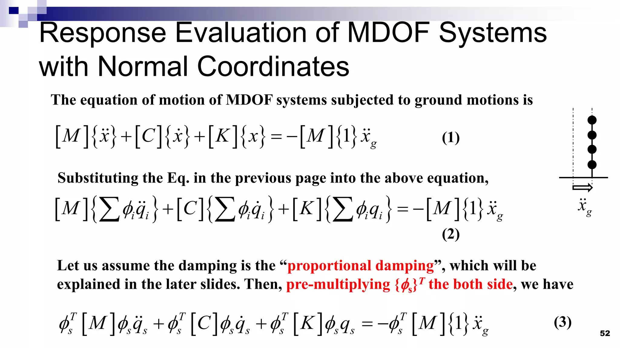
The equation of motion of MDOF systems subjected to ground motions is
           
1 g
M x C x K x M x
   
Let us assume the damping is the “proportional damping”, which will be
explained in the later slides. Then, pre-multiplying {s}T the both side, we have
g
x
(1)
Substituting the Eq. in the previous page into the above equation,
           
1
i i i i i i g
M q C q K q M x
  
   
  
(2)
        
1
T T T T
s s s s s s s s s s g
M q C q K q M x
      
    (3)
Response Evaluation of MDOF Systems
with Normal Coordinates

53. 53
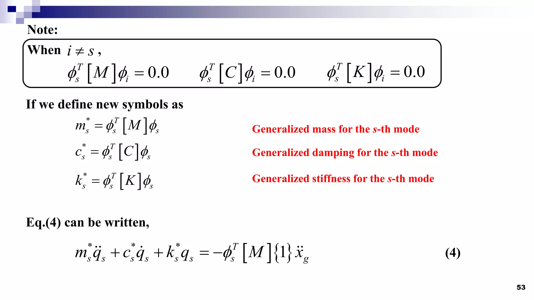
Note:
  0.0
T
s i
M
  
When ,
i s

  0.0
T
s i
C
     0.0
T
s i
K
  
If we define new symbols as
 
* T
s s s
m M
 

 
* T
s s s
c C
 

 
* T
s s s
k K
 

Eq.(4) can be written,
Generalized mass for the s-th mode
Generalized damping for the s-th mode
Generalized stiffness for the s-th mode
  
* * *
1
T
s s s s s s s g
m q c q k q M x

    (4)

54. 54
    
1
T T
s s s
M M
   

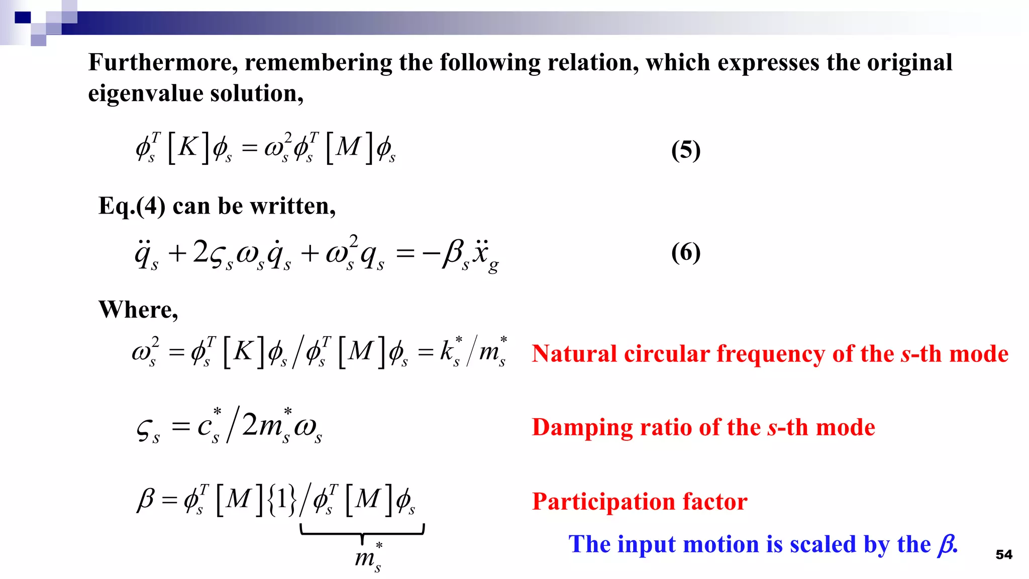
Furthermore, remembering the following relation, which expresses the original
eigenvalue solution,
   
2
T T
s s s s s
K M
    
 (5)
Eq.(4) can be written,
2
2
s s s s s s s g
q q q x
   
    (6)
Participation factor
The input motion is scaled by the .
Where,
* *
2
s s s s
c m
 
 Damping ratio of the s-th mode
   
2 * *
T T
s s s s s s s
K M k m
    
  Natural circular frequency of the s-th mode
*
s
m

55. 55
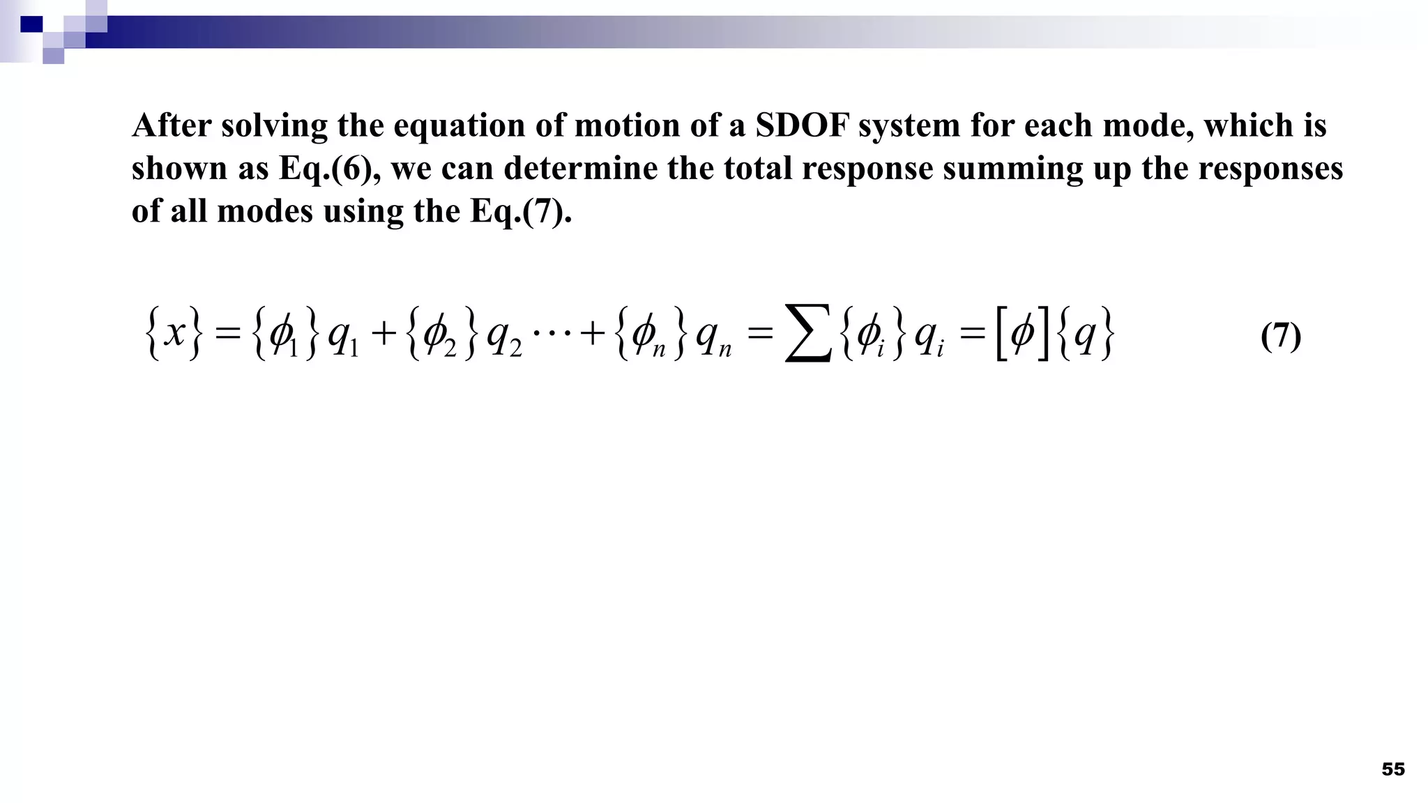
After solving the equation of motion of a SDOF system for each mode, which is
shown as Eq.(6), we can determine the total response summing up the responses
of all modes using the Eq.(7).
            
1 1 2 2 n n i i
x q q q q q
    
    
 (7)

56. Modal Analysis
56
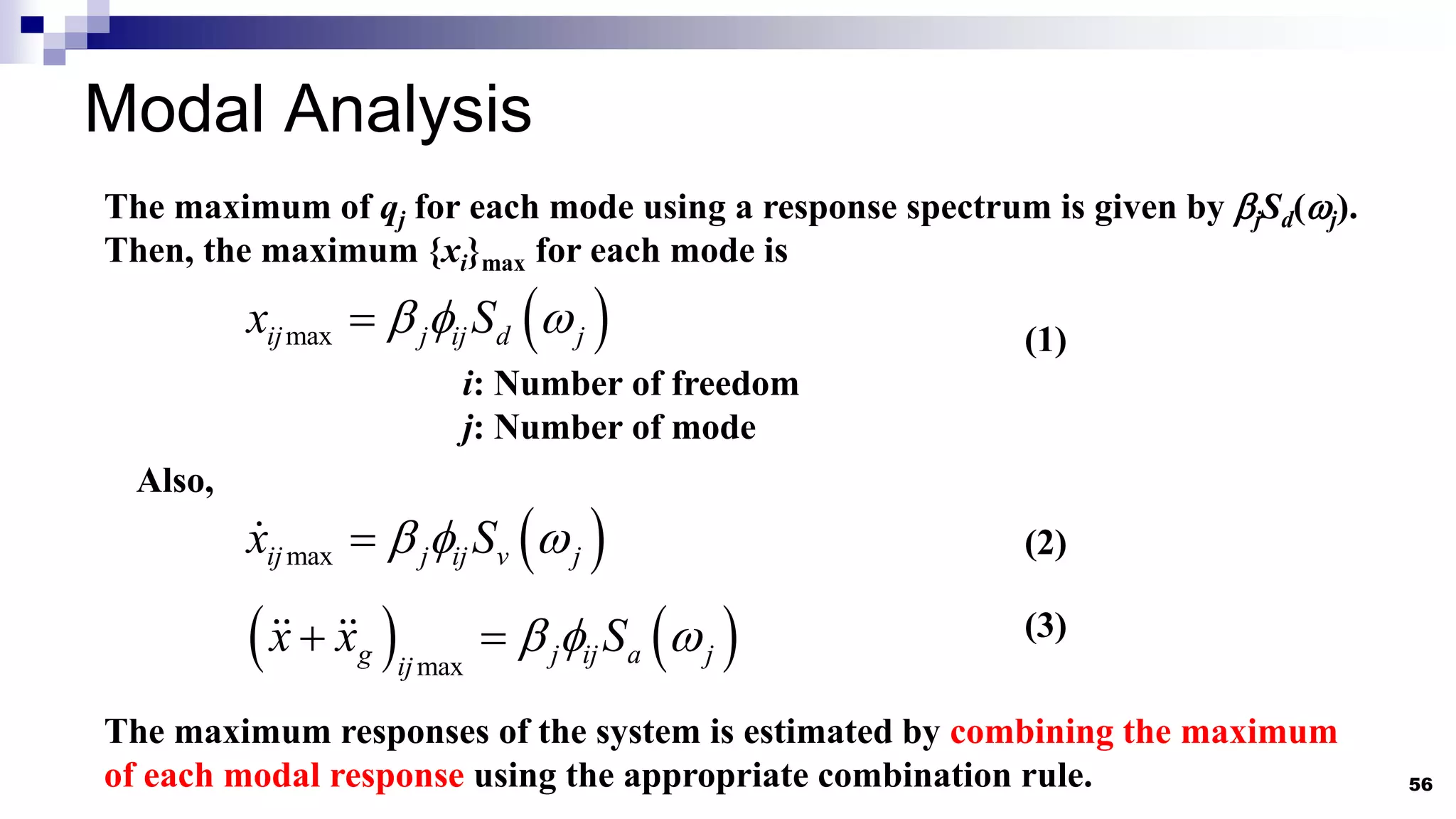
The maximum of qj for each mode using a response spectrum is given by jSd(j).
Then, the maximum {xi}max for each mode is
 
max
ij j ij d j
x S
  
 (1)
i: Number of freedom
j: Number of mode
The maximum responses of the system is estimated by combining the maximum
of each modal response using the appropriate combination rule.
Also,
 
max
ij j ij v j
x S
  

   
max
g j ij a j
ij
x x S
  
 
(2)
(3)

57. 57
[SRSS]: Square Root of Sum of Squares
 
 
2
max( ) 1
n
i SRSS j ij d j
j
x S
  

 
[CQC]: Complete Quadratic Combination
 
   
 
max( ) 1 1
n n
i CQC j ij d j jk k ik d k
j k
x S S
      
 
  
: Factor for estimating correlation between natural frequencies

58. Additional Topic:
Proportional Damping
58
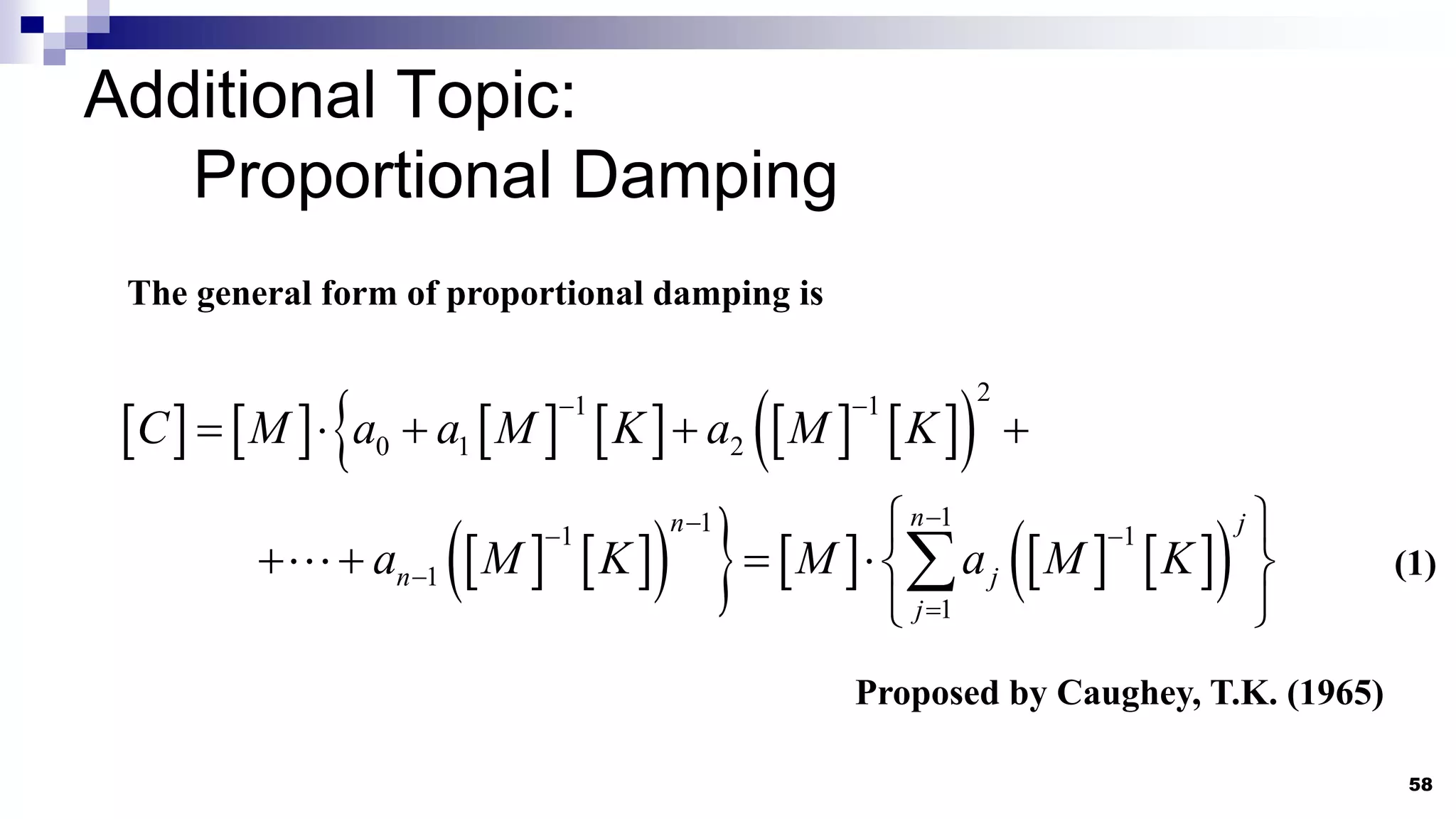
The general form of proportional damping is
       
    
 
2
1 1
0 1 2
C M a a M K a M K
 
    
   
        
 
1
1
1 1
1
1
n
n j
n j
j
a M K M a M K


 


 
    
 

Proposed by Caughey, T.K. (1965)
(1)

59. 59
* *
2
s s s s
c m
 

 
* T
s s s
m M
 

Let us calculate the damping ratio for the s-th mode.
Where,  
* T
s s s
c C
 

(2)
Substituting the general form of [C] into the above equation,
 
* 2 4 2 2 *
0 1 2 1
( ) 2
n
s s s s n s s s
m a a a a m
    


  
 
3 2 1
0 1 2 1
1 2 n
s s s n s
a a a a
    

   (3)
Then
2 4 2( 1)
0 1 1
1 1 1
2 4 2( 1)
1 2 2
2 2 2
2 4 2( 1)
2
1
2
1
2
1
n
n
n
n n n
n n n
a
a
a
 
  
 
  
 
  



     
     
   
  
   
     
     
     
 
(4)

60. 60
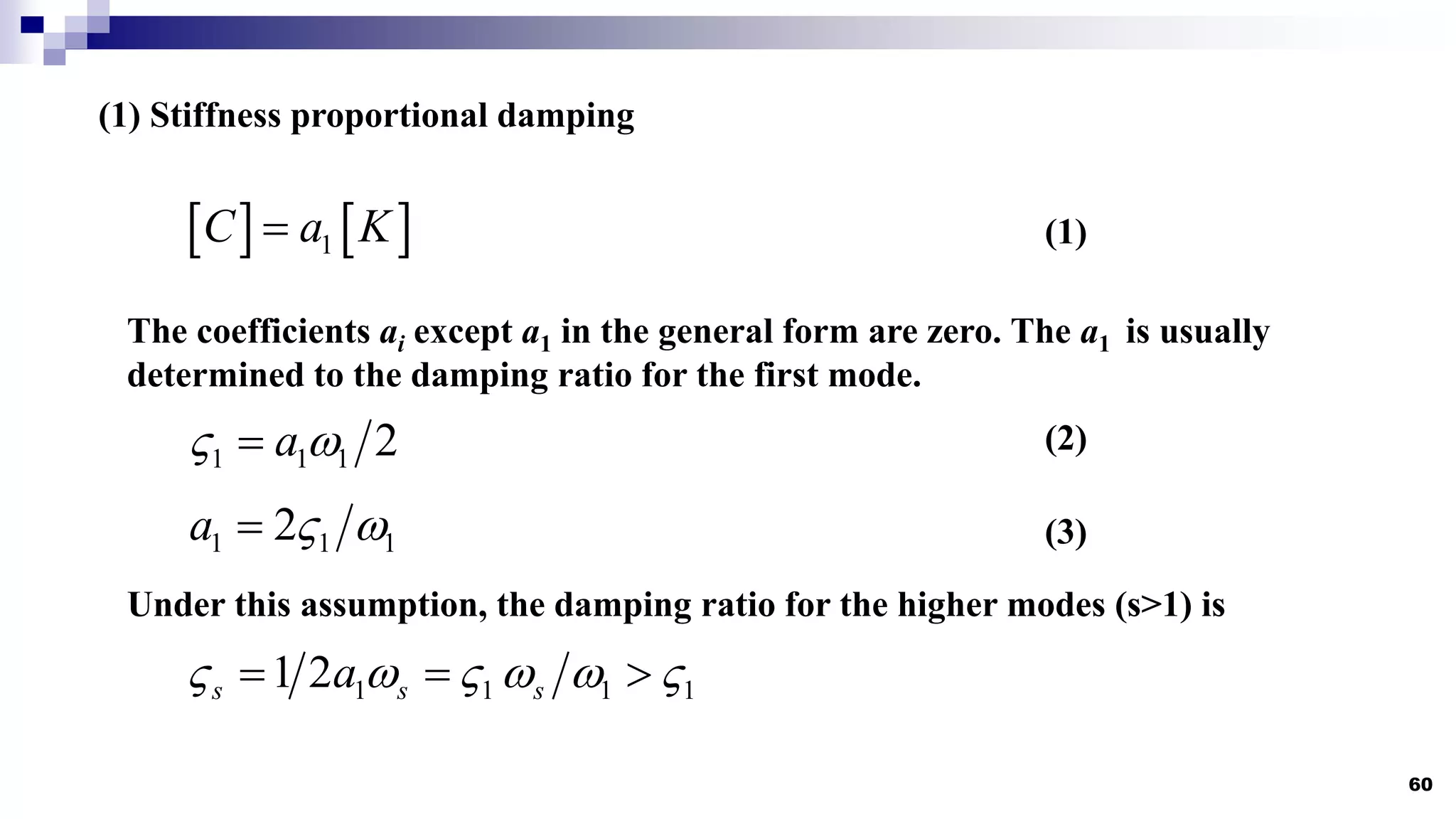
(1) Stiffness proportional damping
   
1
C a K

The coefficients ai except a1 in the general form are zero. The a1 is usually
determined to the damping ratio for the first mode.
1 1 1
2
a  

(1)
(2)
Under this assumption, the damping ratio for the higher modes (s>1) is
1 1 1 1
1 2
s s s
a
     
  
(3)
1 1 1 2
a
 


61. 61
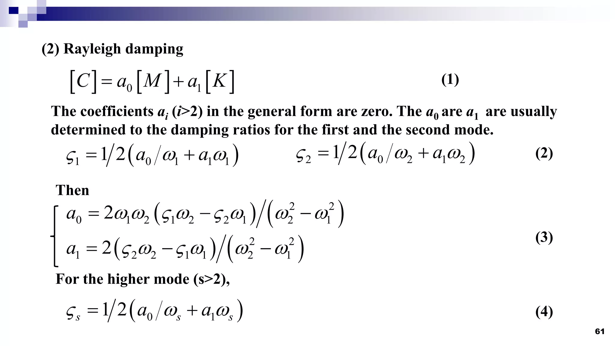
(2) Rayleigh damping
     
0 1
C a M a K
 
The coefficients ai (i>2) in the general form are zero. The a0 are a1 are usually
determined to the damping ratios for the first and the second mode.
 
1 0 1 1 1
1 2 a a
  
   
2 0 2 1 2
1 2 a a
  
 
   
2 2
0 1 2 1 2 2 1 2 1
2
a        
  
   
2 2
1 2 2 1 1 2 1
2
a      
  
Then
For the higher mode (s>2),
 
0 1
1 2
s s s
a a
  
 
(1)
(2)
(3)
(4)