It is machine learning ppt based on classifications.

Classification Task
2
Decision Rules :
If Outlook =“Overcast” then PlayGolf=“Yes”
If Outlook =“Sunny” and Windy=“True” then PlayGolf=“No”
Outlook=“Rainy”, Temp=“Mild”, Humidity=“High” , Windy=“False”,
PlayGolf =?

3
 Classification
 Predicts categorical class labels (discrete or nominal)
 Classifies data (constructs a model) based on the
training set and the values (class labels) and uses it in
classifying new data
 Prediction
 Models continuous-valued functions, i.e., predicts
unknown or missing values
Classification vs. Prediction

Classifying Something Into
Predefined Set Of
Categories/Class Labels

Classification Problem Types
 Binary
 Gender Detection – Male, Female
 Quant Trading – Up Day, Down Day
 Fraud Detection – Fraud, Not Fraud
 Multi-Class
 Weather Forecasting – Cloudy, Sunny, Rainy

Classification Problem Statement
 Given a problem instance, Assign a label to the problem
instance
 A name – Gender Detection
 A time of day – Weather Forecasting
 A trading day – Quant Trading
 A transaction – Fraud Detection

Solving Classification Problem
12
Name
(Problem
Instance)
Classifier Male/
Female
(Class Label)
What is inside
the Black Box?

The Black Box?
 Could be completely opaque – Neural Networks
 Could contain a set of if then rules – Decision Trees
 Could be a set of mathematical equations that we can
understand – Logistic regression, Naïve Bayes

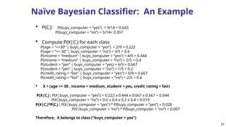
Classification: Definition
 Given a collection of records (training set )
 Each record is characterized by a tuple ([x],y), where [x] is the
attribute set and y is the class label

x: attribute, predictor, independent variable, input

y: class, response, dependent variable, output
 Task:
 Learn a model that maps each attribute set [x] into one of the
predefined class labels y
14

15
Classification—A Two-Step Process
 Model construction:
 Each tuple/sample is assumed to belong to a predefined
class, as determined by the Class label attribute
 Set of tuples used for model construction is Training set
 Model is represented as classification rules, decision
trees, or mathematical formulae

 Model Evaluation: for validating the accuracy of the model
 Estimate accuracy of the model

Set of tuples used for testing the model - Test set

Result from the model is compared with Known label of test sample

Accuracy - % of test set samples that are correctly classified by the
model

Test set - independent of training set, otherwise over-fitting will
occur
 Model usage: for classifying future or unknown objects
 If the accuracy is acceptable in Model Evaluation phase - model is used
to classify data tuples whose class labels are not known
16

17
Process (1): Model Construction
Training
Data
NAME RANK YEARS TENURED
Mike Assistant Prof 3 no
Mary Assistant Prof 7 yes
Bill Professor 2 yes
Jim Associate Prof 7 yes
Dave Assistant Prof 6 no
Anne Associate Prof 3 no
Classification
Algorithms
IF rank = ‘professor’
OR years > 6
THEN tenured = ‘yes’
Classifier
(Model)

18
Process (2): Using the Model in Prediction
Classifier
Testing
Data
NAME RANK YEARS TENURED
Tom Assistant Prof 2 no
Merlisa Associate Prof 7 no
George Professor 5 yes
Joseph Assistant Prof 7 yes
Unseen Data
(Jeff, Professor, 4)
Tenured?

19
Issues: Data Preparation
 Data cleaning
 Preprocess data in order to reduce noise and handle
missing values
 Relevance analysis (feature selection)
 Remove the irrelevant or redundant attributes
 Data transformation
 Generalize and/or normalize data

20
Issues: Evaluating Classification Methods
 Accuracy
 classifier accuracy: predicting class label
 predictor accuracy: guessing value of predicted attributes
 Speed
 Time to construct the model (training time)
 Time to use the model (classification/prediction time)
 Robustness: handling noise and missing values
 Scalability: efficiency in disk-resident databases
 Interpretability
 understanding and insight provided by the model
 Other measures : Goodness of rules, such as, decision tree size or
compactness of classification rules

Decision Tree Induction
 Three Popular Algorithms
 ID3 (Iterative Dichotomiser) – J. Ross Quinlan
 C4.5 (Successor of ID3)
 CART (Classification and Regression Trees)
– binary decision trees
22

23
Decision Tree Induction: Training Dataset
age income student credit_rating buys_computer
<=30 high no fair no
<=30 high no excellent no
31…40 high no fair yes
>40 medium no fair yes
>40 low yes fair yes
>40 low yes excellent no
31…40 low yes excellent yes
<=30 medium no fair no
<=30 low yes fair yes
>40 medium yes fair yes
<=30 medium yes excellent yes
31…40 medium no excellent yes
31…40 high yes fair yes
>40 medium no excellent no
Example of
Quinlan’s ID3
(Iterative
Dichoto-miser)

24
Output: A Decision Tree for “buys_computer”
age?
student? credit rating?
<=30 >40
no yes yes
yes
31..40
no
fair
excellent
yes
no

25
Algorithm for Decision Tree Induction- Basic
Strategies
 Basic algorithm (a greedy algorithm)
 Tree is constructed in a top-down recursive divide-and-conquer
manner
 At start, all the training examples are at the root
 Attributes are categorical (if continuous-valued, they are discretized in
advance)
 Tuples are partitioned recursively based on selected attributes
 Split attributes are selected on the basis of a heuristic or statistical
measure (e.g., information gain)
 Conditions for stopping partitioning
 All samples for a given node belong to the same class
 No remaining attributes for further partitioning – majority voting is
employed for classifying the leaf
 No more samples/tuples left in the table

Example
Income Student Credit_Reating Buys_
Computer
Mediu
m
No Fair Yes
Low Yes Fair Yes
Low Yes Excellent No
Mediu
m
Yes Fair Yes
Mediu
m
No Excellent No
26
Student
Ye
s
No
Income Credit
Rating
Buy-
Computer
Low Fair Yes
Low Excellent No
Medium Fair Yes
Income Credit
Rating
Buy-
Computer
Medium Fair Yes
Medium Excellent No

Algorithm for Decision Tree Induction
 Generate_decision_tree(D, attribute List)
 Create a node N
 If samples in D are all of the same class, C then

Return N as a leaf node labeled with the class C
 If attribute-list is empty then

Return N as a leaf node labeled with most common class in sample D
 Select split-attribute, the attribute with highest info gain from attribute-list
 Label node N with split-attribute
 If split-attribute is discrete-valued and multiway splits allowed then
 attribute-list attribute-list - split attribute
 For each outcome j of splitting_criterion
 For each known value ai of test-attribute

Grow a branch from node N for the condition test-attribute=ai

Let si be the set of samples in samples for which test-attribute=ai

If si is empty then
 Attach a leaf labeled with the most common class in samples

Else attach the node returned by generate_decision_tree(si, attribute-list)
27

Age Salary Degree Buys_
Computer
Young <25K UG Yes
Middle >=25K PG No
Middle <25K UG Yes
Young <25K PG No
Young >=25K PG Yes
28
<25K >=25K
Age Degree Buy-
Computer
Young UG Yes
Middle UG Yes
Young PG No
Age Degree Buy-
Computer
Middle PG No
Young PG Yes
Salary

29
<25K >=25K
Age Buy-
Computer
Young Yes
Middle Yes
Age Degree Buy-
Computer
Middle PG No
Young PG Yes
Salary
Degree
Age Buy-
Computer
Young No
UG
PG

30
<25K >=25K
Age Degree Buy-
Computer
Middle PG No
Young PG Yes
Salary
Degree
YES NO
UG PG

Notations
 D – set of class-labeled tuples (training set)
 m – number of distinct class labels Ci (i=1…m)
 Ci,D - set of tuples of class Ci in D
 |D| - no. of tuples in D
 |Ci,D| - no. of tuples in Ci,D
31

32
Training Dataset (Input)

33
Attribute Selection Measure:
Information Gain (ID3/C4.5)
 Select the attribute with the highest information gain
 Let pi be the probability that an arbitrary tuple in D belongs to
class Ci, estimated by |Ci, D|/|D|
 Expected information (entropy) needed to classify a tuple in D:
 Information needed (after using A to split D into v partitions)
to classify D:
 Information gained by branching on attribute A
(D)
Info
Info(D)
Gain(A) A


)
(
log
)
( 2
1
i
m
i
i p
p
D
Info 




34
Sample Database

35
Attribute Selection: Information Gain
g Class P: buys_computer = “yes” = 9
g Class N: buys_computer = “no” = 4
940
.
0
)
14
5
(
log
14
5
)
14
9
(
log
14
9
)
5
,
9
(
)
( 2
2 



I
D
Info
Information needed to classify D after using age
to classify into 3 partitions is :

Age (<=30)
Income Student Credit_Reating Buys_Computer
High No Fair No
High No Excellent No
Medium No Fair No
Low Yes Fair Yes
Medium Yes Excellent Yes
36

Age (>40)
Income Student Credit_Reating Buys_Computer
Medium No Fair Yes
Low Yes Fair Yes
Low Yes Excellent No
Medium Yes Fair Yes
Medium No Excellent No
37

38
Information Gain of Age
Age Yes No
<=30 2 3
31..40 4 0
>40 3 2
= (5/14) 0.971 +(4/14) 0 +(5/14) 0.971
= 0.694
)
3
,
2
(
14
5
I means “age <=30” has 5 out of 14 samples,
with 2 yes’es and 3 no’s.
246
.
0
)
(
)
(
)
( 

 D
Info
D
Info
age
Gain age
Information needed to classify D after using age to classify into 3
partitions

39
Income Yes No
low 3 1
medium 4 2
high 2 2
Student Yes No
no 3 4
yes 6 1
Credit_rating Yes No
fair 6 2
excellent 3 3

Information Gain
 Gain(age) = 0.246
 Gain(income) = 0.029
 Gain(student) = 0.151
 Gain(credit_rating) = 0.048
40
Attribute Age is selected as split attribute

41
OUTLOOK TEMP(F) HUMIDITY(%) WINDY CLASS
Sunny 79 90 True No play
Sunny 56 70 False Play
Sunny 79 75 True play
sunny 60 90 True No play
Overcast 88 88 False play
Overcast 63 75 True play
Overcast 88 95 False play
Rain 78 60 False play
Rain 66 70 False No play
Rain 68 60 True No play
Sunny 70 75 False No Play
Overcast 68 80 True play
Rain 74 70 True Play
Rain 70 65 False Play
Exercise
Temperature Humidity
< 60 Cool <60 Less
(60-85] Normal (60-80] Medium
>=85 Hot >=80 High

42
Computing Information-Gain for
Continuous-Value Attributes
 For continuous-valued attribute, A :
 Must determine the best split point for A
 Sort the value A in increasing order
 Typically, the midpoint between each pair of adjacent
values is considered as a possible split point
 (ai+ai+1)/2 is the midpoint between the values of ai and ai+1
 The point with the minimum expected information
requirement for A is selected as the split-point for A
 Split:
 D1 is the set of tuples in D satisfying A split-point,
≤
and D2 is the set of tuples in D satisfying A > split-

43
Gain Ratio for Attribute Selection (C4.5)
 Information gain measure is biased towards attributes with a
large number of values
 Uses gain ratio to overcome the problem (normalization to
information gain)
 GainRatio(A) = Gain(A)/SplitInfo(A)
 Ex.
 gain_ratio(income) = 0.029/1.557 = 0.019
 Attribute with the maximum gain ratio is selected as the splitting
attribute
)
|
|
|
|
(
log
|
|
|
|
)
( 2
1 D
D
D
D
D
SplitInfo
j
v
j
j
A 

 

=1.557
Gain(income)=0.029

44
Gini index – Attribute Selection Measure
 Used in CART algorithm
 Measures the impurity of D, a data partition or set of training tuples
 If a data set D contains tuples from n classes, gini index, gini (D) is
defined as
where pj is the probability that a tuple belongs to class Cj in D
and is estimated by |Cj,D|/|D|
 Gini index considers a binary split for each attribute




n
j
p j
D
gini
1
2
1
)
(

Gini index (CART, IBM IntelligentMiner)
 To determine the best split on A, examine all possible subsets that can be formed using
the known values of A
 For Ex., income has 3 values , low, medium and high.
 Possible subsets :

{low, medium, high},
 {low, medium} , {low,high} ,
 {medium, high}, {low}, {medium},
 {high}, {}
 Power set and empty set need not be considered.
 For v distinct values, 2v
– 2 possible ways to form two partitions of the data D, based on
binary split on A
45

46
 If a data set D is split on A into two subsets D1 and D2, the gini
index gini (D) is defined as
 Reduction in Impurity:
 The attribute provides the smallest ginisplit(D) (or the largest
reduction in impurity) is chosen to split the node
)
(
)
(
)
( D
gini
D
gini
A
gini A



)
(
|
|
|
|
)
(
|
|
|
|
)
( 2
2
1
1
D
gini
D
D
D
gini
D
D
D
giniA



47
 Ex. D has 9 tuples in buys_computer = “yes” and 5 in “no”
 Suppose the attribute income partitions D into 10 in D1: {low,
medium} and 4 in D2:{high}
gini{medium,high} = 0.450 = gini{low}
gini{low,high} = 0.458 = gini{medium}
459
.
0
14
5
14
9
1
)
(
2
2
















D
gini
Best Split :
gini{low, medium} and gini{high}
Reduction in impurity :
gini income {low,medium} = 0.016
gini {medium,high} =0.009
gini {low,high} = 0.001




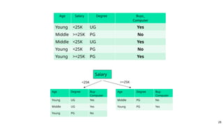
 Evaluating Attribute age, {youth, senior} and {middle_aged} is
the best split with Gini index 0.357.
 Attribute student and credit_rating (binary valued)
gives Gini index values 0.367 and 0.429
respectively.
 Reduction in impurity for best split :
 Gini(income){low,medium} = 0.016
 Gini(age) {youth, senior} = 0.102 [max. reduction in impurity]
 Gini(student) = 0.092
 Gini(credit_rating)=0.030
 So age with two branches {youth, senior} and
{middle_aged} will be grown.
48





49
Comparing Attribute Selection Measures
 The three measures, in general, return good results but
 Information gain:

biased towards multivalued attributes
 Gain ratio:

tends to prefer unbalanced splits in which one partition
is much smaller than the others
 Gini index:

biased to multivalued attributes

has difficulty when # of classes is large

tends to favor tests that result in equal-sized partitions
and purity in both partitions

Attribute Selection Measure
50
)
(
log
)
( 2
1
i
m
i
i p
p
D
Info 



)
(
|
|
|
|
)
(
1
j
v
j
j
A D
I
D
D
D
Info 


(D)
Info
Info(D)
Gain(A) A


)
|
|
|
|
(
log
|
|
|
|
)
( 2
1 D
D
D
D
D
SplitInfo
j
v
j
j
A 

 

GainRatio(A) =
Gain(A)/SplitInfo(A)




n
j
p j
D
gini
1
2
1
)
(
)
(
)
(
)
( D
gini
D
gini
A
gini A



)
(
|
|
|
|
)
(
|
|
|
|
)
( 2
2
1
1
D
gini
D
D
D
gini
D
D
D
giniA


Information Gain Gain Ratio
Gini Index

Overfitting and Tree Pruning
51
• Overfitting: An induced tree may overfit the training
data
• Too many branches, some may reflect anomalies due to noise
or outliers
• Poor accuracy for unseen samples
• Unpruned and Pruned Tree

52
Two approaches to avoid Overfitting
 Prepruning: Halt tree construction early—do not split a node if this
would result in the Goodness Measure (Statsitical Significance, information
gain, Gini index, etc.) falling below a Threshold
 Difficult to choose an appropriate threshold
 Postpruning: Remove branches from a “fully grown” tree—get a
sequence of progressively pruned trees
 A subtree at a given node is pruned by removing its branches and
replacing it with a leaf.
 Leaf is labeled with the most frequent class among the subtree

Cost Complexity pruning
 In CART, cost complexity of a tree ( a function of number of leaves) and error rate (% of
tuples misclassified) of the tree is considered.
 Cost Complexity Computation
 Start from the bottom of the tree.
 For each internal node, N, compute the cost complexity of the subtree at N, and the
cost complexity of the subtree at N if it were to be pruned(i.e., replaced by a leaf node)
 If pruning the subtree at node N result in smaller cost complexity, then the subtree is
pruned.
 Use a set of data different from the training data to decide which is the “best pruned tree”
53

55
Bayesian Classification: Why?
 A statistical classifier: performs probabilistic prediction, i.e., predicts class membership
probabilities
 Foundation: Based on Bayes’ Theorem.
 Performance: A simple Bayesian classifier, naïve Bayesian classifier, has comparable
performance with decision tree and selected neural network classifiers
 Incremental: Each training example can incrementally increase/decrease the probability
that a hypothesis is correct — prior knowledge can be combined with observed data
 Standard: Even when Bayesian methods are computationally intractable, they can provide
a standard of optimal decision making against which other methods can be measured

Bayes Theorem
56
X = age =31..40, income = medium
H = X buys computer ? Or P(H/X)
H/C1 = Yes H/C2 = No

57
Bayesian Theorem: Basics
 X – a data sample (“evidence”): class label is unknown
 H - hypothesis that X belongs to class C
 Classification - determine P(H|X)(posterior probability of H,
conditioned on X), the probability that the hypothesis holds given the
observed data sample X
 P(H) (prior probability), the initial probability
 E.g., X will buy computer, regardless of age, income, …
 P(X): probability that sample data is observed
 P(X|H) (posterior probability of X, conditioned on H), the probability of
observing the sample X, given that the hypothesis holds
 E.g., Given that X will buy computer, the prob. that X is 31..40,
medium income

58
Bayesian Theorem
 Given training data X, posteriori probability of a
hypothesis H, P(H|X), follows the Bayes theorem
 Informally, this can be written as
posteriori = likelihood x prior/evidence
 Predicts X belongs to Ci iff the probability P(Ci|X) is the
highest among all the P(Ck|X) for all the k classes
 Practical difficulty: require initial knowledge of many
probabilities, significant computational cost
)
(
)
(
)
|
(
)
|
(
X
X
X
P
H
P
H
P
H
P 

59
Towards Naïve Bayesian Classifier
 D - training set of tuples and their associated class
labels
 Each tuple is represented by an n-D attribute vector
X = (x1, x2, …, xn)
 Let there are be m classes, C1, C2, …, Cm.
 Classification is to derive the maximum posteriori, i.e.,
the maximal P(Ci|X)
 This can be derived from Bayes’ theorem
 Since P(X) is constant for all classes, only
)
(
)
(
)
|
(
)
|
(
X
X
X
P
i
C
P
i
C
P
i
C
P 
)
(
)
|
(
)
|
(
i
C
P
i
C
P
i
C
P X
X 

60
Derivation of Naïve Bayes Classifier
 Simplified Assumption: Attributes are conditionally independent :
Where X = (x1, x2, …, xn)
 Reduces the computation cost: Only counts the class distribution
 If Ak is categorical, P(xk|Ci) is the # of tuples in Ci having value xk
for Ak divided by |Ci, D| (# of tuples of Ci in D)
 If Ak is continuous-valued, P(xk|Ci) is usually computed based on
Gaussian distribution with a mean μ and standard deviation σ
and P(xk|Ci) is
)
|
(
...
)
|
(
)
|
(
1
)
|
(
)
|
(
2
1
Ci
x
P
Ci
x
P
Ci
x
P
n
k
Ci
x
P
Ci
P
n
k







X
2
2
2
)
(
2
1
)
,
,
( 








x
e
x
g
)
,
,
(
)
|
( i
i C
C
k
x
g
Ci
P 


X

61
Naïve Bayesian Classifier: Training Dataset
Class:
C1:buys_computer = ‘yes’
C2:buys_computer = ‘no’
Data sample X =
(age <=30, Income =
medium, Student = yes
Credit_rating = Fair)
age income student
credit_rating
buys_computer

62
Naïve Bayesian Classifier: An Example

P(Ci): P(buys_computer = “yes”) = 9/14 = 0.643
P(buys_computer = “no”) = 5/14= 0.357

Compute P(X|Ci) for each class
P(age = “<=30” | buys_computer = “yes”) = 2/9 = 0.222
P(age = “<= 30” | buys_computer = “no”) = 3/5 = 0.6
P(income = “medium” | buys_computer = “yes”) = 4/9 = 0.444
P(income = “medium” | buys_computer = “no”) = 2/5 = 0.4
P(student = “yes” | buys_computer = “yes) = 6/9 = 0.667
P(student = “yes” | buys_computer = “no”) = 1/5 = 0.2
P(credit_rating = “fair” | buys_computer = “yes”) = 6/9 = 0.667
P(credit_rating = “fair” | buys_computer = “no”) = 2/5 = 0.4
 X = (age <= 30 , income = medium, student = yes, credit_rating = fair)
P(X|Ci) : P(X|buys_computer = “yes”) = 0.222 x 0.444 x 0.667 x 0.667 = 0.044
P(X|buys_computer = “no”) = 0.6 x 0.4 x 0.2 x 0.4 = 0.019
P(X|Ci)*P(Ci) : P(X|buys_computer = “yes”) * P(buys_computer = “yes”) = 0.028
P(X|buys_computer = “no”) * P(buys_computer = “no”) = 0.007
Therefore, X belongs to class (“buys_computer = yes”)

Exercise
63
X = (age > 40, Income = low, Student = no, Credit_Rating = Excellent)
X = (age = 31..40, Income = low, Student = no, Credit_Rating = Excellent)

64
Avoiding the 0-Probability Problem
 Naïve Bayesian prediction requires each conditional prob. be
non-zero. Otherwise, the predicted prob. will be zero
 Ex. Suppose a dataset with 1000 tuples, income=low (0), income=
medium (990), and income = high (10),
 Use Laplacian correction (or Laplacian estimator)
 Adding 1 to each case
Prob(income = low) = 1/1003
Prob(income = medium) = 991/1003
Prob(income = high) = 11/1003
 The “corrected” prob. estimates are close to their
“uncorrected” counterparts



n
k
Ci
xk
P
Ci
X
P
1
)
|
(
)
|
(

65
Naïve Bayesian Classifier: Comments
 Advantages
 Easy to implement
 Good results obtained in most of the cases
 Disadvantages
 Assumption: class conditional independence,
therefore loss of accuracy
 Practically, dependencies exist among variables

E.g., hospitals: patients: Profile: age, family history, etc.
Symptoms: fever, cough etc., Disease: lung cancer, diabetes,
etc.

Dependencies among these cannot be modeled by Naïve
Bayesian Classifier
 How to deal with these dependencies?
 Bayesian Belief Networks

It is machine learning ppt based on classifications.

More Related Content

Similar to It is machine learning ppt based on classifications.

Recently uploaded

It is machine learning ppt based on classifications.

Editor's Notes