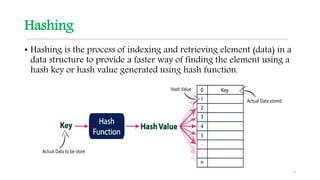
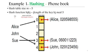
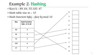
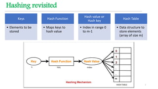
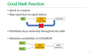
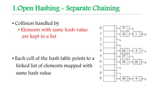
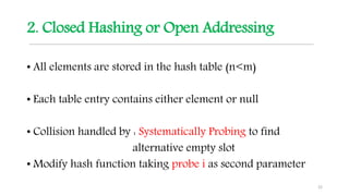
This document discusses hashing techniques for indexing and retrieving elements in a data structure. It begins by defining hashing and its components like hash functions, collisions, and collision handling. It then describes two common collision handling techniques - separate chaining and open addressing. Separate chaining uses linked lists to handle collisions while open addressing resolves collisions by probing to find alternate empty slots using techniques like linear probing and quadratic probing. The document provides examples and explanations of how these hashing techniques work.

1. HASHING
BY
B.HEMALATHA , AP-CSE
VELAMMAL ENGINEERING COLLEGE

2. Topics to be discussed
•HASHING
•HASH FUNCTION
•COLLISION
•COLLISION HANDLING
•REHASHING
•EXTENDIBLE HASHING
•APPLICATIONS
2

3. Hashing
• Hashing is the process of indexing and retrieving element (data) in a
data structure to provide a faster way of finding the element using a
hash key or hash value generated using hash function.
3

4. Example 1: Hashing - Phone book
• Hash table size m = 5
• Hash function h(k) = (length of the key k) mod 5
4

5. Example 2: Hashing
• Keys k = 89, 64, 35,100, 47
• Hash table size m = 10
• Hash function h(k) = (key k) mod 10
5
Key Hash function
h(k) = k % 10
89 9
64 4
35 5
100 0
47 7
0 100
1
2
3
4 64
5 35
6
7 47
8
9 89
5

6. Why hashing?
• Many applications deal with lots of data
 eg. Search engines and web pages
Requirement : Time Critical Look Ups
• Implemented with Data structures like
a. Arrays and Lists
b. BST
c. Hash Tables
Solution: Hash tables with Hashing improves searching
with CONSTANT TIME
6
linear time for look ups O(n)
look-ups in near constant time
O(1)
linear time for look ups O(n)

7. Hashing revisited
Keys
• Elements to be
stored
Hash Function
• Maps keys to
hash value
Hash value or
Hash key
• Index in range 0
to m-1
Hash Table
• Data structure to
store elements
(array of size m)
7

8. Hash Function
• Mapping of keys to indices of a hash table is called hash function
Keys Hash key in range 0 to TableSize m-1
• Comprises of 2 maps
Hash code map
Compression map
Key Integer Hash Index in range (0…,m-1)
where m is size of hash table
8
mapping
Hash code
map
Compression
map

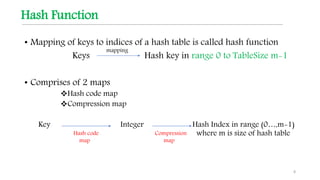
9. Hash Function
• A hash function h maps keys of a given type to integers in a
fixed interval [0,……,m - 1]
h(k) hash value of k
9

10. Good Hash Function
• Quick to compute
• Map equal keys to equal indices
• Distributes keys uniformly throughout the table
• Minimises probability of COLLISION
10
KEY HASH
FUNCTION
HASH KEY
KEY 1
HASH
FUNCTION
SAME
HASH KEY
KEY 2

11. Hash Function
• Deal with non-integer keys
• Integer cast: interpret the bits of the key as integer
• Sum of ASCII value of characters in string as integer
• Component sum: partition the bits of the key into parts of fixed length
combine the components to one integer using sum
11

12. Hash Function
• Mid-square method: pick m bits from the middle of k2
• Division method : h(k) = k mod m
where k = key and m=TableSize
Note: If m is prime it ensures uniform
distribution
12

13. Hash Function for Division method
13

14. Hash Table
For TableSize = m and hashing function h(k) = k mod m
• m - prime (good) ensures uniform distribution
• m – power of 2 (bad) gives keys with same ending with same hash
value
LOAD FACTOR - measure of how full the table is
• α = 𝑛
𝑚
• Load factor mostly α < 1
• α grows - hash table becomes slower
• α bounded – maintains O(1) 14

15. Collision
• Two keys map to the same hash value
15
KEY 1
HASH
FUNCTION
SAME
HASH KEY
KEY 2

16. Example - Collision
Insert keys 89, 18, 49, 58, 69
16
Index Keys
0
1
2
3
4
5
6
7
8
9 89
Index Keys
0
1
2
3
4
5
6
7
8 18
9 89
Index Keys
0
1
2
3
4
5
6
7
8 18
9 89
Insert 89 Insert 18 Insert 49
h(k)= k mod Tablesize
= k % 10
h(89)=89 % 10
= 9
h(18) = 8 % 10
= 8
h(49) = 9 % 10
= 9
Collision occurs as
Slot 9 occupied by
89

17. Collision Handling
17

18. 1.Open Hashing - Separate Chaining
• Collision handled by
• Elements with same hash value
are kept in a list
• Each cell of the hash table points to a
linked list of elements mapped with
same hash value
18

19. Example - Separate Chaining
Insert keys 89, 27, 49, 55, 69 ,45
Key Hash function
h(k) = k % 10
89 9
27 7
49 9
55 5
69 9
45 5
19
h(k)= k mod Tablesize
= k % 10
0
1
2
3
4
5
6
7
8
9
45
49 69
55
27
89

20. Separate Chaining - Operations
• Search - hash function h(k) determines which list to traverse
- search the appropriate list
• Insert - hash function h(k) determines which list to insert
- check the list
- new element inserted at the front of the list
- duplicate element : an extra data member kept and
incremented
• Delete - hash function h(k) determines which list to traverse
- search the appropriate list
- delete the node in the list
20

21. Separate Chaining
• Advantage - Insert more elements
- Simple to implement
• Disadvantage
• Search an element in linked list O(n)
• Expensive - extra data structure, links, more unused
memory
• Cache performance of chaining is not good as keys are
stored using a linked list.
21

22. 2. Closed Hashing or Open Addressing
• All elements are stored in the hash table (n<m)
• Each table entry contains either element or null
• Collision handled by : Systematically Probing to find
alternative empty slot
• Modify hash function taking probe i as second parameter
22

23. Open Addressing or Closed Hashing
• When collision occurs probing is done
Modify hash function for probing
hi(k) =( h( k ) + f ( i ) ) mod Tablesize with f(0) = 0
• Function f is the collision resolution strategy
• Probing : Slots h0(k), h1(k), h2(k), . . . are tried in succession
to find alternative slot until an empty slot is found
23

24. Open
Addressing
Linear
Probing
Quadratic
Probing
Double
Hashing
24

25. Linear Probing
Collision resolution strategy
Function f(i) = i where i is the probe parameter
Hashing function
hi(k) = [ h(k) + f(i) ] mod TableSize
= [ h(k) + i ] mod TableSize
Probe sequence: i iterating from 0 until alternative empty slot
0th probe = h(k) mod TableSize
1th probe = [ h(k) + 1] mod TableSize
2th probe = [ h(k) + 2] mod TableSize
. . .
ith probe = [ h(k) + i ]mod TableSize 25

26. Linear probing
Insert keys 89, 18, 49, 58, 69
26
Index Keys
0
1
2
3
4
5
6
7
8
9 89
Index Keys
0
1
2
3
4
5
6
7
8 18
9 89
Index Keys
0 49
1
2
3
4
5
6
7
8 18
9 89
Insert 89 Insert 18 Insert 49
hi(k) =[ h( k ) + i ] mod Tablesize
= [ h( k ) + i ] % 10
i=0
h0(89)
=[ h(89)+0 ] % 10
=[ 9+0 ] % 10
= 9
i=0
h0(18)
=[ h(18)+0 ] % 10
=[ 8+0 ] % 10
= 8
i=0
h0(49)
=[ h(49)+0 ] % 10
=[ 9+0 ] % 10
= 9
i=1
h1(49)
=[ h(49)+1 ]%10
=[9 +1] % 10
= 0
Collision occurs as
Slot 9 occupied by 89

27. Linear probing ………….. Contd.
Insert keys 89, 18, 49, 58, 69
27
Index Keys
0 49
1 58
2
3
4
5
6
7
8 18
9 89
Index Keys
0 49
1 58
2 69
3
4
5
6
7
8 18
9 89
Insert 58 Insert 69
i=0
h0(58)
=[ h(58)+0] % 10
=[ 8+0 ] % 10
= 8
(Collision)
i=0
h0(69)
=[ h(69)+0 ] % 10
= 9
(Collision)
i=1
h1(58)
=[ h(58)+1 ] % 10
=[ 8+1 ] % 10
= 9
(Collision)
i=2
h2(58)
=[ h(58)+2 ] % 10
=[ 8+2 ] % 10
= 0
(Collision)
i=3
h3(58)
=[ h(58)+3) % 10
=[ 8+3 ] % 10
= 1
i=1
h1(69)
=[ h(69)+1 ] % 10
= 0
(Collision)
i=2
h2(69)
=[ h(69)+2 ] % 10
= 1
(Collision)
i=3
h3(69)
=[ h(69)+3 ] % 10
= 2
hi(k) =[ h( k ) + i ] mod Tablesize
= [ h( k ) + i ] % 10

28. Insertion Routine
LinearProbeInsert(k)
if (table is full) error
probe = h(k) // probe= location
while (table [probe] occupied)
probe = (probe+1) mod m
table [probe] = k
28

29. Lookup in linear probing
• Continue looking at successive locations (Probing)
till k is successfully found
an empty location encountered
Search 55 : h(55) = 5
Search 6 : h(6) = 6
29
65 46 17 55
0 1 2 3 4 5 6 7 8 9
65 46 17 55
0 1 2 3 4 5 6 7 8 9
FOUND 55
EMPTY
UNSUCCESSFUL
SEARCH

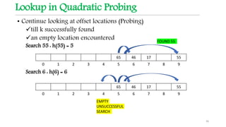
30. Search Routine
LinearProbeSearch(k)
if (table is empty) error
probe = h(k) // probe= location
while (table [probe] occupied and table [probe]!=k )
probe = (probe+1) mod m
if table [probe] = k
return probe
else
not found
30

31. Deletion in Linear Probing
• Search for key to be deleted
• Delete the key
• Set location with marker / flag (X)
Rehash if more markers
Delete 15
31
65 46 15 58
0 1 2 3 4 5 6 7 8 9
65 46 X 58
0 1 2 3 4 5 6 7 8 9
h(k)+1 h(k)+2

32. Linear Probing
• Advantage - Uses less memory than chaining
- Simple to implement
- Best cache performance
- For any α < 1, successful insertion
• Disadvantage – Primary clustering leads to more no. of
probes
- Performance quickly degrades for α > ½
for look ups
32
0 30
1 90
2 41
3
4
5 55
6
7
8 68
9 49

33. Quadratic Probing
Collision resolution strategy
Function f(i) = i2 where i is the probe parameter
Hashing function
hi(k) = [ h(k) + f(i) ] mod TableSize
= [ h(k) + i2 ] mod TableSize
Probe sequence: i iterating from 0
0th probe = h(k) mod TableSize
1th probe = [ h(k) + 1 ] mod TableSize
2th probe = [ h(k) + 4 ] mod TableSize
3rd probe = [ h(k) + 9 ] mod TableSize
. . . ith probe = [ h(k) + i2
] mod TableSize 33

34. Quadratic Probing
Insert keys 89, 18, 49, 58, 69
34
Index Keys
0
1
2
3
4
5
6
7
8
9 89
Index Keys
0
1
2
3
4
5
6
7
8 18
9 89
Index Keys
0 49
1
2
3
4
5
6
7
8 18
9 89
Insert 89 Insert 18 Insert 49
hi(k) = [ h ( k ) + i2 ] mod Tablesize
= [ h ( k ) + i2 ] % 10
i=0
h0(89)
=[ h(89)+ 02]%10
=[ 9 + 0] % 10
= 9
i=0
h0(18)
=[ h(18)+ 02]%10
=[ 8 + 0] % 10
= 8
i=0
h0(49)
=[ h(49)+ 02
]%10
= 9
i=1
h1(49]
=[ h(49)+ 12
]%10
= 0
Collision occurs as
Slot 9 occupied by 89

35. Quadratic probing ………….. Contd.
Insert keys 89, 18, 49, 58, 69
35
Index Keys
0 49
1
2 58
3
4
5
6
7
8 18
9 89
Index Keys
0 49
1
2 58
3 69
4
5
6
7
8 18
9 89
Insert 58 Insert 69
i=0
h0(58)= [ h(58)+ 02]%10
= 8
(Collision)
i=0
h0(69) = [ h(69)+ 02]%10
= 9
(Collision)
i=1
h1(58) = [ h(58)+ 12]%10
= 9
(Collision)
i=2
h2(58)= [ h(58)+ 22]%10
= 2
i=1
h1(69) = [ h(69)+ 12
]%10
= 0
(Collision)
i=2
h2(69) = [ h(69)+ 22]%10
= 3
hi(k) = [ h ( k ) + i2 ] mod Tablesize
= [ h ( k ) + i2 ] % 10

36. Lookup in Quadratic Probing
• Continue looking at offset locations (Probing)
till k successfully found
an empty location encountered
Search 55 : h(55) = 5
Search 6 : h(6) = 6
36
65 46 17 55
0 1 2 3 4 5 6 7 8 9
65 46 17 55
0 1 2 3 4 5 6 7 8 9
FOUND 55
EMPTY
UNSUCCESSFUL
SEARCH

37. Deletion in Quadratic Probing
• Search for key to be deleted
• Delete the key
• Set location with marker/flag (x)
Rehash if more markers
Delete 15
37
65 46 58 15
0 1 2 3 4 5 6 7 8 9
65 46 58 X
0 1 2 3 4 5 6 7 8 9
h(k)+1
h(k)+4

38. Quadratic Probing
• Advantage
• Avoids Primary clustering
• Disadvantage
• Secondary clustering – probing the same sequence in looking
for an empty location
• If table size is not a prime number, probes will not try all locations in
the table
38

39. Double Hashing
• Uses 2 hash functions h1(k) and h2(k)
• h1(k) is first position to check keys
h1(k) = k mod TableSize
• h2(k) determines offset
h2(k) = R – (k * mod R) where R is a prime smaller than
TableSize
• Collision resolution strategy
Function f(i) = i ∗ h2(k)
• Hashing function
hi(k)= [ h1(k) + f(i) ] mod TableSize
hi(k)= [ h1(k) + i ∗ h2(k) ] mod TableSize
39
hi(k)= [ h1(k) + f(i) ] mod TableSize

40. Double Hashing
Hashing function
hi(k)= [ h1(k) + i ∗ h2(k) ] mod TableSize
where h1(k) = k mod TableSize and h2(k)=R – (k * mod R)
Probe sequence: i iterating from 0
0th probe = h(k) mod TableSize
1th probe = [ h1(k) + 1∗ h2(k) ] mod TableSize
2th probe = [ h1(k) + 2 ∗ h2(k) ] mod TableSize
3rd probe = [ h1(k) + 3 ∗ h2(k) ] mod TableSize
. . .
ith probe = [ h1(k) + i ∗ h2(k) ] mod TableSize
40

41. Double Hashing
Insert keys 89, 18, 49, 58, 69
41
hi(k)= [ h1(k) + i ∗ h2(k) ] mod TableSize
= [ h1(k) + i ∗ h2(k) ] % 10
KEY 89 18 49 58 69
h1(k)=k % 10 9 8 9 8 9
h2(k) = R – ( k mod R )
=7 – ( k % 7 )
2 3 7 5 1
hi(k) = ( h1(k) + i * h2(k) ) % 10
For i=0
h0(89)
= (9+0*2) % 10
= 9
h0(18)
= (8+0*3) % 10
= 8
h0(49)
= (9+0*7) % 10
= 9
h0(58)
= (8+0*7) % 10
= 8
h0(69)
= (9+0*7) % 10
= 9
i=1
h1(49)
= (9+1*7) % 10
= 6
h1(58)
= (8+1*7) % 10
= 3
h1(69)
= (9+1*7) % 10
= 0
0 1 2 3 4 5 6 7 8 9
69 58 49 18 89
HASH TABLE

42. Double Hashing
DoubleHashingInsert(k)
if (table is full) error
probe=h1(k) ; offset=h2(k) // probe= location
while (table[probe] occupied)
probe=(probe+offset) mod m
table[probe]=k
42

43. Double Hashing
• If the table size is not prime, it is possible to run out of alternative
locations prematurely
• Advantages
• Distributes key more uniformly than linear probing
• Reduces clustering
• Allows for smaller tables (higher load factors) than linear or
quadratic probing, but at the expense of higher costs to compute
the next probe
• Disadvantage
• As table fills up performance degrades
• Time-consuming to compute two hash functions
• Poor cache performance
43

44. Rehashing
• Rehashing done when
• Table is mostly full operations are getting slow
• Insertion fails
• Load factor exceeds its bound
• Steps for rehashing
• Build another Hash table with increased TableSize
• Hash code regenerated with hash function
44

45. Example - Rehashing
45
TableSize m= 17
Hash table with linear probing
with input 13, 15, 6, 24
Hash table with linear
probing
after 23 is inserted
TableSize m= 7
AFTER
REHASHING

46. Extendible Hashing
• When the table gets too full
• Rehashing done - expensive
• Extendible hashing can be done
• Extendible hashing
• Allows search in 2 disk accesses
• Insertions also require few disk
accesses
• Dynamic hashing method Uses
• Directory
• Buckets
46

47. Extendible Hashing
47

48. Extendible Hashing
• Directory
• Array with 2𝑑 entries where d is dictionary levels called the global
depth
• Global depth d - # of bits used from each hash value
• d no. of bits are used to choose the directory entry for key
insertion and searching
• Can grow, but its size is always a power of 2
• Entry has bucket address (pointers) which is used to access buckets
• Multiple directory entries may point to the same bucket
• Bucket
• has a local depth d’ that indicates how many of the d bits of the hash
value are actually used to indicate membership in the bucket
• Keys are stored in buckets
48

49. Example – Extendible Hashing Searching
49
4 Directory
entries
pointers
d = global
depth
𝑑′= local depth hash function h(k)=k mod 4
To search 15
h(k)=15% 4 = 3 (11 in b)
which points to bucket D

50. Extendible Hashing Insertion
• Assume each hashed key is a sequence of four binary digits.
➯Store values 0001, 1001, 1100
As d= 1 first bit of key is used
for choosing directory
look up
0001, 1001, 1100
50
Bucket A
Bucket B

51. Extendible Hashing Insertion Contd…
51
Bucket A
Bucket B

52. Extendible Hashing Insertion Contd…
52
Insert 1111 Directory grows one level

53. Overflow Handling during Insertion
53

54. Overflow Handling during Insertion
• If overflow occurs
• Case 1 : Local depth of the overflown bucket = Global depth before
split
• Directory doubles (grows) and global depth incremented (d ++)
• Bucket is split into two and local depth incremented (d′ ++)
• Keys redistributed in the split buckets
• Case 2 : Local depth of the overflown bucket < Global depth before
split
• Bucket is split into two and local depth incremented (d′ ++)
• No change in directory ( d remains same)
54

55. Example - Overflow Handling during Insertion
d = global depth
incremented
𝑑′
= local depth incremented
𝑑′= local depth incremented
h(63)= 63 % 4 = 3 ( 11 in b) which points to bucket D which overflows
As d=d’
Case 1 : Directory doubled and bucket D is split
BUCKET
D is split
Inserting 63
h(63)= 63 % 8 = 7 ( 111 in b)
which points to bucket D′

56. Example - Extendible Hashing Insertion
56
After
inserting 17
and 13
h(13) = 13 % 8 =5 (101)
Points bucket B’
h(17) = 17 % 8 =1 (001)
Points bucket B

57. Extendible Hashing Deletion
• If deletions cause a bucket to be substantially less than
full
•Find a buddy bucket to collapse
•Two buckets are buddies if:
• They are at the same depth.
• Their initial bit strings are the same.
• Collapsing them will fit all records in one bucket
• Collapse if a bucket is empty
57

58. Example - Extendible Hashing Deletion
58

59. Extendible Hashing
• Advantages
• Key search takes only one disk access if the directory can be
kept in RAM, otherwise it takes two
• Disadvantages
• Doubling the directory is a costly operation
• Directory may outgrow main memory
59

60. Applications
• Compilers use hash tables to keep track of declared variables
• On-line spell checkers
• “hash” an entire dictionary
• Quickly check if words are spelled correctly in constant
time
60

61. Applications
61
Password checkers

62. Thank You