The document discusses greedy algorithms and provides examples. It begins with an overview of greedy algorithms and their properties. It then provides a sample problem (traveling salesman) and shows how a greedy approach can provide an iterative solution. The document notes advantages and disadvantages of greedy algorithms and provides additional examples, including optimal binary tree merging and the knapsack problem. It concludes with describing algorithms for optimal solutions to these problems.

1. Greedy Algorithms
Assistant Professor. Mary‘am
Department Of Computer Science
University Of South-Asia
Lahore Cantonment
1

2. 05/24/16
Group Members Details
2
Hafiz Furqan Tahir
B-18298
Ghufran Qamar
B- 20142
ALL GROUP MEMBERS
Sadiq Sultan
B-18031
Abdul Wahab Ahmed
B-18108
PRESENTERS

3. Greedy Algorithm Short
Explanation
3
Greedy Algorithms:
Many real-world problems are optimization problems in that
they attempt to find an optimal solution among many
possible candidate solutions

4. 05/24/16
What is Greedy Algorithm?
•
In the hard words: A greedy algorithm is
an algorithm that follows the problem solving
heuristics of making the locally optimal choice at
each stagewith the hope of finding a global
optimum.
(source: http://en.wikipedia.org/wiki/Greedy_algorithm)
•
Simplify: Choose the best choice that ‘reachable’
at current state
4

5. 05/24/16
Sample Usage of Greedy
•
For better explanation we use old simple
problem: Travelling Salesman Problem:
5

6. 05/24/16
TSP
•
The Problem is how to travel from city A and
visit all city on the map, then back to city A
again.
•
The rules: you only visit each city once and you
can’t pass through any traversed path.
6

7. 05/24/16
Solution:
•
Find the shortest path from city A(start) to any
other city.
•
Because the nearest city is B, so we go to B
7
BA

8. 05/24/16
•
From B, we find any other city but A(because A
has been visited) that has nearest path. So we
choose C:
Keep tuning on…
8
BA
C

9. 05/24/16
•
From C, we look to nearest city again, but don’t
look for A and B, because both has been visited.
So we choose D.
Soon end…
9
BA
C D

10. 05/24/16
•
At this node(D), we can’t go to any city, because
all neighbor of D has been visited. We go back to
first city(A).
•
And that was how to solve TSP problem.
10
BA
C D

11. 05/24/16
Advantage of Greedy
•
Greedy is easy to be implemented. Just search
the best choice from the current state that
‘reachable’ (has any paths or any connections).
•
In simple case, greedy often give you the best
solution.
11

12. 05/24/16
Drawback of Greedy
•
In large and complex case, greedy doesn’t always
give you the best solution, because it’s just
search and take the best choice that you can
reach from the current state.
•
It takes longer time than any other algorithms
for big case of problem
12

13. 05/24/16Graph (and Digraph) Traversal techniques:
Given a (directed) graph G = (V, E), determine all nodes
that are connected from a given node v via a
(directed) path.
The are essentially two graph traversal algorithms, known
as Breadth-first search (BFS) and depth-first search
(DFS), both of which can be implemented
efficiently.
BFS: From node v, visit each of its neighboring nodes in
sequence, then visit their neighbors, etc., while
avoiding repeated visits.
DFS: From node v, visit its first neighboring node and all
its neighbors using recursion, then visit node v’s
second neighbor applying the same procedure, until
all v’s neighbors are visited, while avoiding repeated
13

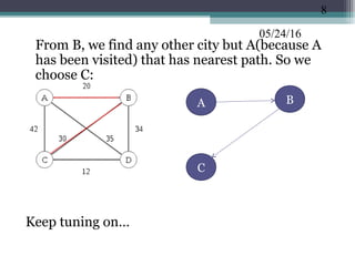
14. 05/24/16
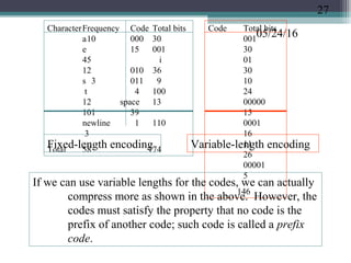
Breadth-First Search (BFS):
BFS(v) // visit all nodes reachable from node v
(1) create an empty FIFO queue
Q, add node v to Q (2) create a
boolean array visited[1..n], initialize all values
to false except for visited[v] to true
(3) while Q is not empty
(3.1) delete a node w from Q
(3.2) for each node z adjacent from
node w if
visited[z] is false then
add node z to Q and set visited[z] to
true
1
2 4
3
5
6
Node search order
starting
with node
1,
including
two nodes
not
reached
The time complexity is O(n+e)
with n nodes and e
edges, if the
adjacency lists are
used. This is because
in the worst case,
each node is added
once to the queue
(O(n) part), and each
of its neighbors gets
14

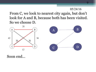
15. 05/24/16
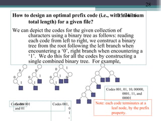
Depth-First Search (DFS):
(1) create a boolean array visited[1..n], initialize all
values to false except for visited[v] to true
(2) call DFS(v) to visit all nodes
reachable via a path
DFS(v)
for each neighboring nodes w of
v do if
visited[w] is false then
set visited[w] to true; call
DFS(w) // recursive call
1
2 5
3 6
4
Node search order
starting with
node 1,
including two
nodes not
reached
The algorithm’s time
complexity is
also O(n+e) using
the same
reasoning as in
the BFS
algorithm.
15

16. 05/24/16Example: To make change for the amount x = 67 (cents).
Use q = x/25 = 2 quarters. The remainder = x – 25q
= 17, which we use d = 17/10 = 1 dime. Then the
remainder = 17 – 10d = 7, so we use n = 7/5 = 1
nickel. Finally, the remainder = 7 – 5n = 2, which
requires p = 2/1 = 2 pennies. The total number of
coins used = q + d + n + p = 6.
Note: The above algorithm is optimal in that it uses the
fewest number of coins among all possible ways to
make change for a given amount. (This fact can be
proven formally.) However, this is dependent on the
denominations of the US currency system. For
example, try a system that uses denominations of 1-
cent, 6-cent, and 7-cent coins, and try to make change
for x = 18 cents. The greedy strategy uses 2 7-cents
and 4 1-cents, for a total of 6 coins. However, the
16

17. 05/24/16A Generic Greedy Algorithm:
(1) Initialize C to be the set of candidate solutions
(2) Initialize a set S = the empty set ∅ (the
set is to be the optimal solution
we are constructing). (3) While C ≠
∅ and S is (still) not a solution do
(3.1) select x from set C using a greedy strategy
(3.2) delete x from C
(3.3) if {x} ∪ S is a
feasible solution, then
S = S ∪ {x} (i.e., add x to set S)
(4) if S is a solution then
return S
(5) else return
failure
In general, a greedy algorithm is efficient because it makes a
sequence of (local) decisions and never backtracks.
17

18. 05/24/16The Knapsack Problem:
Given n objects each have a weight wi and a value vi , and
given a knapsack of total capacity W. The problem is
to pack the knapsack with these objects in order to
maximize the total value of those objects packed
without exceeding the knapsack’s capacity. More
formally, let xi denote the fraction of the object i to be
included in the knapsack, 0 ≤ xi ≤ 1, for 1 ≤ i ≤ n.
The problem is to find values for the xi such that
Note that we may assume because otherwise, we
would choose xi = 1 for each i which would be an
obvious optimal solution.
∑∑ ≤
==
n
i
ii
n
i
ii vxWwx
11
maximized.isand
∑ >
=
n
i
i Ww
1
18

19. 05/24/16
19
There seem to be 3 obvious greedy strategies:
(Max value) Sort the objects from the highest value to the
lowest, then pick them in that order.
(Min weight) Sort the objects from the lowest weight to the
highest, then pick them in that order.
(Max value/weight ratio) Sort the objects based on the
value to weight ratios, from the highest to the lowest, then
select.
Example: Given n = 5 objects and a knapsack capacity W =
100 as in Table I. The three solutions are given in Table II.
w 10 20 30 40 50
v 20 30 66
40 60 v/w
2.0 1.5 2.2 1.0
1.2Table I
select xi value
Max vi 0 0 1 0.5 1
146 Min wi 1 1 1
1 0 156 Max vi/wi
1 1 1 0 0.8 164Table II
19

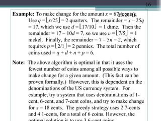
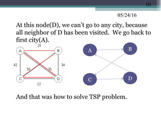
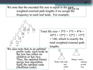
20. 05/24/16The Optimal Knapsack Algorithm:
Input: an integer n, positive values wi and vi , for 1
≤ i ≤ n, and another positive value W.
Output: n values xi such that 0 ≤ xi ≤ 1 and
Algorithm (of time complexity O(n lgn))
(1) Sort the n objects from large to small based on
the ratios vi/wi . We assume the arrays w[1..n]
and v[1..n] store the respective weights and
values after sorting. (2) initialize array x[1..n] to
zeros. (3) weight = 0; i = 1
(4) while (i ≤ n and
weight < W) do (4.1)
if weight + w[i] ≤ W then x[i] = 1
(4.2) else x[i] = (W – weight) / w[i]
(4.3) weight = weight + x[i]
* w[i] (4.4) i++
∑∑ ≤
==
n
i
ii
n
i
ii vxWwx
11
maximized.isand
20

21. 05/24/16Optimal 2-way Merge patterns and Huffman Codes:
Example. Suppose there are 3 sorted lists L1, L2, and L3, of
sizes 30, 20, and 10, respectively, which need to be
merged into a combined sorted list, but we can merge
only two at a time. We intend to find an optimal
merge pattern which minimizes the total number of
comparisons. For example, we can merge L1 and L2,
which uses 30 + 20 = 50 comparisons resulting in a
list of size 50. We can then merge this list with list L3,
using another 50 + 10 = 60 comparisons, so the total
number of comparisons is 50 + 60 = 110.
Alternatively, we can merge lists L2 and L3, using 20 +
10 = 30 comparisons, the resulting list (size 30) can
then be merged with list L1, for another 30 + 30 = 60
comparisons. So the total number of comparisons is
30 + 60 = 90. It doesn’t take long to see that this
latter merge pattern is the optimal one.
21

22. 05/24/16
Binary Merge Trees: We can depict the merge patterns
using a binary tree, built from the leaf nodes (the
initial lists) towards the root in which each merge of
two nodes creates a parent node whose size is the sum
of the sizes of the two children. For example, the two
previous merge patterns are depicted in the following
two figures:
Merge L1 and L2, then with L3
30 20
50 10
60
1020
30 30
60
Merge L2 and L3, then with L1
merge cost = sum of all weighted external path lengths
Cost = 30*2 +
20*
2 +
10*
1 =
110
Cost = 30*1 +
20*
2 +
10*
2 =
90
22

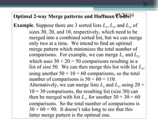
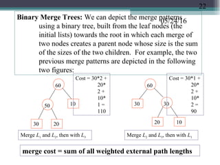
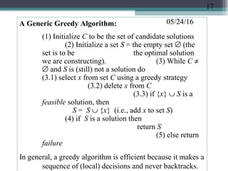
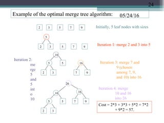
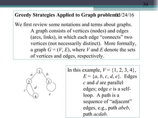
23. 05/24/16Optimal Binary Merge Tree Algorithm:
Input: n leaf nodes each have an integer size, n ≥ 2.
Output: a binary tree with the given leaf nodes
which has a minimum total weighted
external path lengths
Algorithm:
(1) create a min-heap T[1..n ] based on the n initial
sizes. (2) while (the heap size ≥ 2) do
(2.1) delete from the
heap two smallest values, call
them a and b, create a parent node of size a + b
for the nodes corresponding to these
two values (2.2) insert the value (a
+ b) into the heap which
corresponds to the node created in Step (2.1)
When the algorithm terminates, there is a single value left in
the heap whose corresponding node is the root of the
optimal binary merge tree. The algorithm’s time
complexity is O(n lgn) because Step (1) takes O(n)
23

24. 05/24/16Example of the optimal merge tree algorithm:
2 3 5 7 9
2 3
5
5 7 9
2 3
5 5
10
7 9
Initially, 5 leaf nodes with sizes
Iteration 1: merge 2 and 3 into 5
Iteration 2:
me
rge
5
and
5
int
o
10
16 Iteration 3: merge 7 and
9 (chosen
among 7, 9,
and 10) into 16
2 3
5
10
5 7 9
16
26
Iteration 4: merge
10 and 16
into 26
Cost = 2*3 + 3*3 + 5*2 + 7*2
+ 9*2 = 57.
24

25. 05/24/16
Proof of optimality of the binary merge tree algorithm:
We use induction on n ≥ 2 to show that the binary merge tree is optimal in that it gives
the minimum total weighted external path lengths (among all possible ways
to merge the given leaf nodes into a binary tree).
(Basis) When n = 2. There is only one way to
merge two nodes. (Induction Hypothesis) Suppose the
merge tree is optimal when there are k leaf nodes, for some k ≥ 2.
(Induction)
Consider (k + 1) leaf nodes. Call them a1, a2, …, and ak+1. We may assume
nodes a1, a2 are of the smallest values, which are merged in the first step of
the merge algorithm into node b. We call the merge tree T, the part
excluding a1, a2 T’ (see figure). Suppose an optimal binary merge tree is S.
We make two observations. (1) If node x of S is a deepest internal node, we
may swap its two children with nodes a1, a2 in S without increasing the total
weighted external path lengths. Thus, we may assume tree S has a subtree S’
with leaf nodes x, a2, …, and ak+1. (2) The tree S’
must be an optimal merge tree for k
nodes x, a2, …, and ak+1. By
induction hypothesis, tree S’ has a
total weighted external path lengths equal
to that of tree T’. Therefore, the total
weighted external path lengths of T
equals to that of tree S, proving the
optimality of T.
T
T’
S
S’
x
a1 a2 a1 a2
b
25

26. 05/24/16Huffman Codes:
Suppose we wish to save a text (ASCII) file on the disk or to
transmit it though a network using an encoding scheme
that minimizes the number of bits required. Without
compression, characters are typically encoded by their
ASCII codes with 8 bits per character. We can do
better if we have the freedom to design our own
encoding.
Example. Given a text file that uses only 5 different letters (a,
e, i, s, t), the space character, and the newline character.
Since there are 7 different characters, we could use 3
bits per character because that allows 8 bit patterns
ranging from 000 through 111 (so we still one pattern
to spare). The following table shows the encoding of
characters, their frequencies, and the size of encoded
(compressed) file.
26

27. 05/24/16
CharacterFrequency Code Total bits
a10 000 30
e 15 001
45 i
12 010 36
s 3 011 9
t 4 100
12 space 13
101 39
newline 1 110
3
Total 58 174
Code Total bits
001
30
01
30
10
24
00000
15
0001
16
11
26
00001
5
146
Fixed-length encoding Variable-length encoding
If we can use variable lengths for the codes, we can actually
compress more as shown in the above. However, the
codes must satisfy the property that no code is the
prefix of another code; such code is called a prefix
code.
27

28. 05/24/16How to design an optimal prefix code (i.e., with minimum
total length) for a given file?
We can depict the codes for the given collection of
characters using a binary tree as follows: reading
each code from left to right, we construct a binary
tree from the root following the left branch when
encountering a ‘0’, right branch when encountering a
‘1’. We do this for all the codes by constructing a
single combined binary tree. For example,
Code 001Codes 001
and 01
Codes 001,
0
1
,
Codes 001, 01, 10, 00000,
0001, 11, and
00001
0
0
1
0
0 1
1
1
0
0
10
1
Note: each code terminates at a
leaf node, by the prefix
property.
28

29. 05/24/16
We note that the encoded file size is equal to the total
weighted external path lengths if we assign the
frequency to each leaf node. For example,
3
‘s’
1
‘n’
4
‘t’
10
‘a’
15
‘e’
12
‘i’
13
‘ ’
Total file size = 3*5 + 1*5 + 4*4 +
10*3 + 15*2 + 12*2 + 13*2
= 146, which is exactly the
total weighted external path
lengths.
We also note that in an optimal
prefix code, each node in
the tree has either no
children or has two.
Thus, the optimal binary
merge tree algorithm
finds the optimal code
(Huffman code).
Node x has only
one
child
y
x
y
x
Merge x and y,
reducin
g total
size
29

30. 05/24/16Greedy Strategies Applied to Graph problems:
We first review some notations and terms about graphs.
A graph consists of vertices (nodes) and edges
(arcs, links), in which each edge “connects” two
vertices (not necessarily distinct). More formally,
a graph G = (V, E), where V and E denote the sets
of vertices and edges, respectively.
1
2 3
4
a b
c
d
e
In this example, V = {1, 2, 3, 4},
E = {a, b, c, d, e}. Edges
c and d are parallel
edges; edge e is a self-
loop. A path is a
sequence of “adjacent”
edges, e.g., path abeb,
path acdab.
30

31. 05/24/16Directed graphs vs. (un-directed) graphs:
If every edge has an orientation, e.g., an edge starting from
node x terminating at node y, the graph is called a
directed graph, or digraph for short. If all edges have
no orientation, the graph is called an undirected graph,
or simply, a graph. When there are no parallel edges
(two edges that have identical end points), we could
identify an edge with its two end points, such as edge
(1,2), or edge (3,3). In an undirected graph, edge
(1,2) is the same as edge (2,1). We will assume no
parallel edges unless otherwise stated.
1
2 3
e
a b
c
d
A directed graph. Edges c and d
are parallel (directed)
edges. Some directed paths
are ad, ebac.
4
31

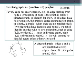
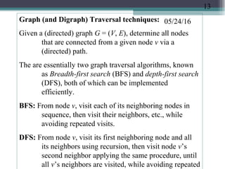
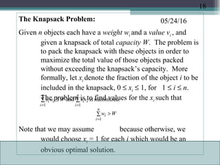
32. 05/24/16Both directed and undirected graphs appear often and naturally
in many scientific (call graphs in program analysis),
business (query trees, entity-relation diagrams in
databases), and engineering (CAD design) applications.
The simplest data structure for representing graphs and
digraphs is using 2-dimensional arrays. Suppose G =
(V, E), and |V| = n. Declare an array T[1..n][1..n] so that
T[i][j] = 1 if there is an edge (i, j) ∈ E; 0 otherwise.
(Note that in an undirected graph, edges (i, j) and (j, i)
refer to the same edge.)
1
4
2 3












0010
0101
1000
0010
1 2 3 4
1
2
3
4
A 2-dimensional
array for the
digraph,
called the
adjacency
matrix.
i
j
32

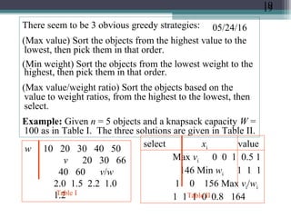
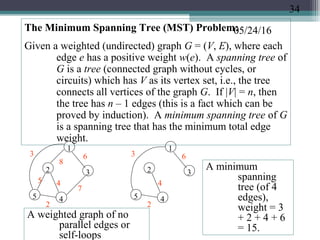
33. 05/24/16Sometimes, edges of a graph or digraph are given a
positive weight or cost value. In that case, the
adjacency matrix can easily modified so that T[i]
[j] = the weight of edge (i, j); 0 if there is no edge
(i, j). Since the adjacency matrix may contain
many zeros (when the graph has few edges,
known as sparse), a space-efficient representation
uses linked lists representing the edges, known as
the adjacency list representation.
1
4
2 3
1
2
3
4
2
4
3 1
2
The adjacency lists for the digraph, which
can store edge weights by adding
another field in the list nodes.
33

34. 05/24/16The Minimum Spanning Tree (MST) Problem:
Given a weighted (undirected) graph G = (V, E), where each
edge e has a positive weight w(e). A spanning tree of
G is a tree (connected graph without cycles, or
circuits) which has V as its vertex set, i.e., the tree
connects all vertices of the graph G. If |V| = n, then
the tree has n – 1 edges (this is a fact which can be
proved by induction). A minimum spanning tree of G
is a spanning tree that has the minimum total edge
weight.
1
4
2 3
5
A weighted graph of no
parallel edges or
self-loops
3
8
6
5 4
2
7
45
3
4
2
1
2 3
6
A minimum
spanning
tree (of 4
edges),
weight = 3
+ 2 + 4 + 6
= 15.
34

35. 05/24/16
Prim’s Algorithm for the Minimum Spanning Tree problem:
Create an array B[1..n] to store the nodes of the MST, and an
array T[1..n –1] to store the edges of the MST. Starting
with node 1 (actually, any node can be the starting node),
put node 1 in B[1], find a node that is the closest (i.e., an
edge connected to node 1 that has the minimum weight,
ties broken arbitrarily). Put this node as B[2], and the
edge as T[1]. Next look for a node connected from either
B[1] or B[2] that is the closest, store the node as B[3],
and the corresponding edge as T[2]. In general, in the kth
iteration, look for a node not already in B[1..k] that is the
closest to any node in B[1..k]. Put this node as B[k+1],
the corresponding edge as T[k]. Repeat this process for n
–1 iterations (k = 1 to n –1). This is a greedy strategy
because in each iteration, the algorithm looks for the
minimum weight edge to include next while maintaining
the tree property (i.e., avoiding cycles). At the end there
are exactly n –1 edges without cycles, which must be a
35

36. 05/24/16
Example: Prim’s MST Algorithm.
5
5 4
2
7
4
2 3
13
8 6
A weighted graph
Step Next edge selected Partial tree
Initially 1
1 (1,5), weight=3
5
1
2 (5,4), weight=2
1
5 4
3 (4,2), weight=4 5
4
2
1
4 (1,3), weight=6 2
1
35
4
3
2
4
6
36

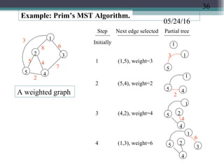
37. 05/24/16An adjacency matrix implementation of Prim’s algorithm:
Input: W[1..n][1..n] with W[i, j] = weight of edge (i, j); set W[i, j] = ∞ if
no edge Output: an MST with tree edges stored in T[1..n –1]
Algorithm:
(1) declare nearest[2..n], minDist[2..n] such that minDistt[i] = the
minimum edge weight connecting node i to any node in partial tree T, and
nearest[i]=the node in T that gives minimum distance for node i.
(2) for i = 2 to n do
nearest[i]=1; minDist[i]=W[i, 1]
(3) for p = 1 to (n –1) do
(3.1) min = ∞
(3.2) for j = 2 to n do
if 0 ≤ minDist[j] < min then
min = minDist[j]; k = j
(3.3) T[p] = edge (nearest[k], k) // selected the
nest edge (3.4) minDist[k] = –1 // a negative
value means node k is “in” (3.5) for j = 2 to n
do // update minDist and nearest values
if W[j, k] < minDist[j] then
minDist[j] = W[j, k]; nearest[j] = k
The time complexity is O(n2
) because Step (3) runs O(n) iterations, each iteration
Tree T
i
nearest[i]
minDist[i]
37

38. 05/24/16The Single-Source Shortest Paths Problem:
Given a directed graph, and a single node called the source.
For each of the remaining nodes, find a shortest
path connected from the source (assuming the
direction of the edges along the paths are respected).
A Greedy algorithm due to Dijkstra which finds
these shortest paths in sequence can be described as
follows: find the shortest among all shortest paths
(from the source), then find the second shortest, etc.,
breaking ties arbitrarily, until all shortest paths are
found. During the process, the collection of all the
shortest paths determined so far form a tree; the next
shortest path is selected by finding a node that is one
edge away from the current tree and has the shortest
distance measured from the source.
38

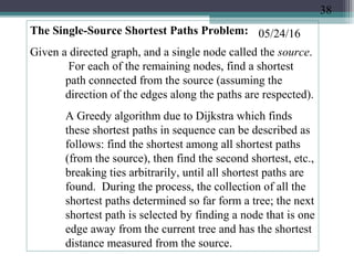
39. 05/24/16Example (Dijkstra’s shortest paths algorithm):
1
2
34
5
A weighted directed
graph,
source node
= 1
10 50
100
10
30
20
50
5
Remaining nodes
and the distances
step tree of shortest
paths from the source
Initially 1 C = [ 2, 3, 4, 5]
D =
[50,30,10
0,10]
Choose
n
o
d
e
5
1
5
[ 2, 3, 4]
[50,
30,
20]
Changed
f
r
o
m
1
0
0
Choose
n
o
d
e
4
1
5
4
[ 2, 3]
[4
0,
30
]
Changed
f
r
o
m
5
0
Choose
n
o
d
e
3
5
4
1
3
[ 2]
[
3
5
]
Changed
f
r
o
m
4
0
Choose
n
o
d
3
1
5
4
2
∅
Shortest paths:
To Path
Distance
5 (1,5) 10
4 (1,5,4)
20
39

40. 05/24/16Implementation of Dijkstra’s algorithm:
Input: W[1..n][1..n] with W[i, j] = weight of edge (i, j); set W[i, j] = ∞ if no
edge Output: an array D[2..n] of distances of shortest paths to each
node in [2..n] Algorithm:
(1) C = {2,3,…,n} // the set of remaining nodes
(2) for i = 2 to n do D[i] = W[1,i] // initialize
distance from node 1 to node i (3) repeat the following n
– 2 times // determine the shortest distances
(3.1) select node v of set C that has the minimum value in array D
(3.2) C = C – {v} // delete node v
from set C (3.3)
for each node w in C do
if (D[v] + W[v, w] < D[w]) then
D[w]
= D[v] + W[v, w] // update D[w] if found shorter path to w1
v
w
W[v,w]
D[v]
D[w]
Tree of
short
est
The algorithm’s time complexity
is O(n2
) because Steps
(1) and (2) each take
O(n) time; Step (3)
runs in O(n) iterations
in which each iteration
runs in O(n) time.
40

41. 05/24/16
Thank’s for
watching
41