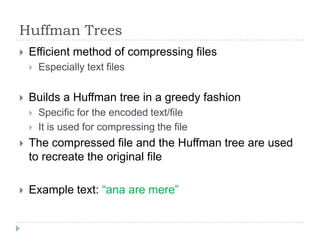
![Example – from CLRS
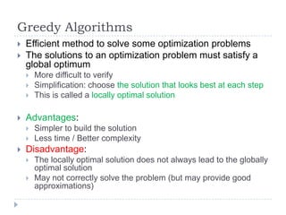
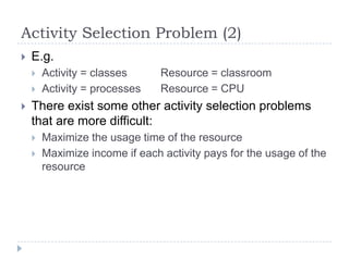
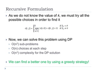
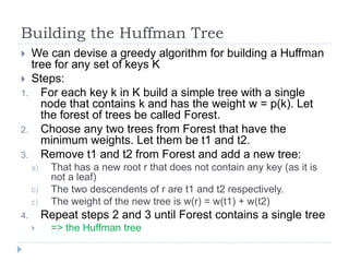
We can devise a greedy solution if we consider the
activities sorted by their finish times
i
1
2
3
4
5
6
7
8
9
s[i] 1
2
4
1
5
8
9
11
13
f[i] 3
5
7
8
9
10
11
14
16
Solution: {a1, a3, a6, a8}
Not unique: {a2, a5, a7, a9}](https://image.slidesharecdn.com/adc5-101118090335-phpapp01/85/Algorithm-Design-and-Complexity-Course-5-8-320.jpg)
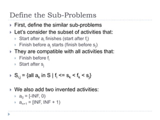
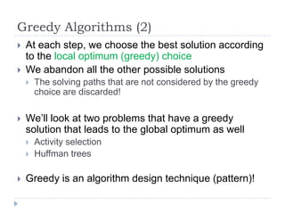
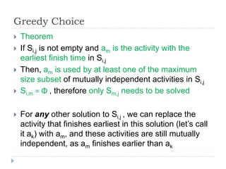
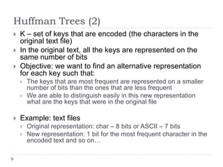
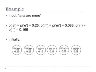
![Optimal Substructure (2)
If an optimal solution to Si,j includes ak, then the subsolutions for Si,k and Sk,j must also be optimal
Ai,j = optimal solution for Si,j
Ai,j = Ai,k U {ak} U Ak,j
If Si,j is not empty
We know ak
c[i, j] = |Ai,j| = maximum size of the subset of
mutually compatible activities in Ai,j
c[i, j] = 0 if i >= j](https://image.slidesharecdn.com/adc5-101118090335-phpapp01/85/Algorithm-Design-and-Complexity-Course-5-12-320.jpg)
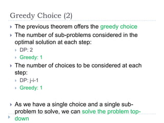
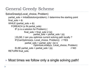
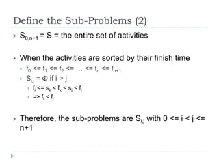
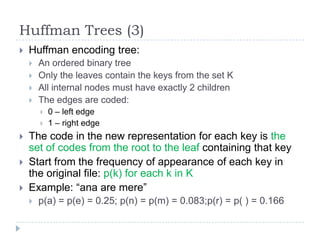
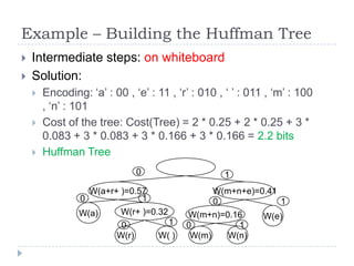
![Recursive Algorithm
Because the greedy algorithm considers the activities sorted by their
finish time, we first need to sort by the finish time!
O(n logn)
RecursiveActivitySelection(s, f, i, n)
m = i +1
WHILE (m <= n AND s[m] < f[i])
m++
// find the activity with the earliest
// start time that starts after activity i finishes
IF (m <= n) THEN
RETURN {am} U RecursiveActivitySelection(s, f, m, n)
RETURN Φ
Initial call: RecursiveActivitySelection(s, f, 0, n)
Complexity: (n) – go through each activity once](https://image.slidesharecdn.com/adc5-101118090335-phpapp01/85/Algorithm-Design-and-Complexity-Course-5-17-320.jpg)
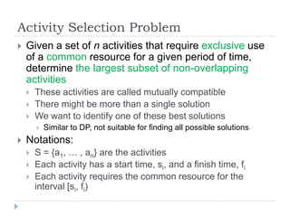
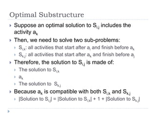
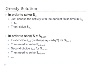
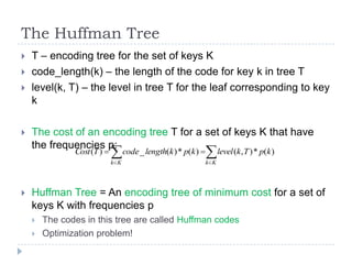
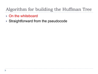
![Iterative Algorithm
Can turn the recursive algorithm into an iterative one
IterativeActivitySelection(s, f, n)
A = {a1}
i=1
FOR (m = 2..n)
IF (s[m] < f[i])
CONTINUE
ELSE
A = A U {am}
i=m
RETURN A
Complexity:
(n) – go once through each activity](https://image.slidesharecdn.com/adc5-101118090335-phpapp01/85/Algorithm-Design-and-Complexity-Course-5-18-320.jpg)
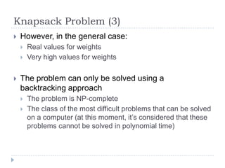
![Knapsack Problem
Given a set on n items:
Which are the items that should be carried in order
to maximize the total value that can be carried in a
knapsack of total weight W?
Values v[i]
Weights w[i]
Optimization problem
Similar to the change-making problem
Given a set of divisions (coins and banknotes for a
currency), find the minimum number of coins and
banknotes needed to change a given amount of money](https://image.slidesharecdn.com/adc5-101118090335-phpapp01/85/Algorithm-Design-and-Complexity-Course-5-31-320.jpg)
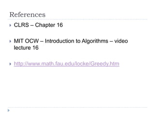
![Knapsack Problem (2)
Can be solved efficiently if:
Are allowed to carry fractions of the items
Fractional knapsack problem
Greedy solution: sort the items according to the ratio v[i]/w[i] and
choose the items in the order of the highest ratio until the
knapsack is full
We are not allowed to carry fractions of the items
Integer (0/1) knapsack problem
But the values for weights and values are relatively small
integers
DP solution: on whiteboard](https://image.slidesharecdn.com/adc5-101118090335-phpapp01/85/Algorithm-Design-and-Complexity-Course-5-32-320.jpg)

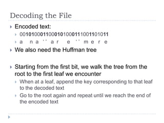
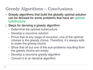
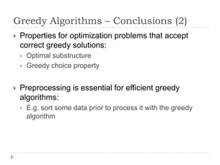
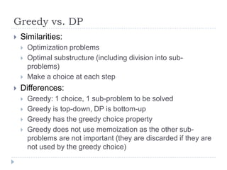
This document provides an overview of greedy algorithms and their use in solving optimization problems. It discusses key aspects of greedy algorithms including making locally optimal choices at each step, optimal substructures, and the greedy choice property. Two problems addressed in detail are the activity selection problem and building Huffman trees. The activity selection problem can be solved optimally using a greedy approach by always selecting the activity with the earliest finish time. Huffman trees provide data compression by assigning codes to characters based on frequency, with more common characters having shorter codes, and can be constructed greedily by repeatedly combining the two subtrees with lowest weight.