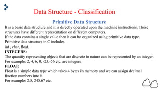
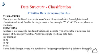
This document provides an introduction to data structures, defining them as organized collections of data and classifying them into primitive (e.g., int, char, float) and non-primitive structures (e.g., arrays, linked lists, stacks, queues, trees, graphs). It further elaborates on memory allocation techniques, including static and dynamic allocation, memory management functions, and recursion methods. Applications and operations of data structures are discussed, emphasizing their relevance in efficiently representing and managing data within computer systems.


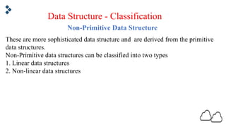
![Non-Primitive Data Structure
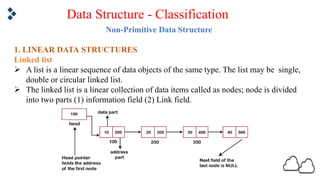
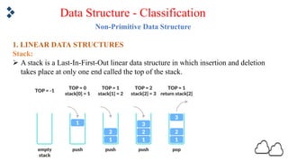
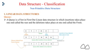
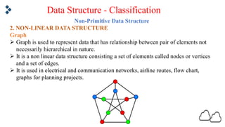
1. LINEAR DATA STRUCTURES
In linear data structure the elements are stored in the memory in a sequential
order and there exists an adjacency relationship between the elements. The
linear data structures are:
Array: Array is a collection of data items of same data type, stored in
consecutive memory location and is referred by common name. It means an
array can contain one type of data, either all integers or characters.
Declaration of an array: int a[n];
Data Structure - Classification](https://image.slidesharecdn.com/unit1-introduction-bca-240429191213-fb7d9793/85/Unit-1-Introduction-to-Data-Structures-BCA-pdf-6-320.jpg)

![MEMORY ALLOCATION
Static Memory Allocation:
v Static memory allocation means we reserve a certain amount of memory by default,
inside our program to use for variables.
v It is fixed in size. It need not grow or shrink in size.
v The standard method of creating an array of 10 integers on the stack is:
v int arr[10];
v This means 10 memory locations are allocated to hold 10 integers. Memory is said to
be allocated statically.
v In real world problems, we do not exactly know how much static data space to declare.
If we declare more static data space, we waste space. If we declare less static data
space, we run out of space.](https://image.slidesharecdn.com/unit1-introduction-bca-240429191213-fb7d9793/85/Unit-1-Introduction-to-Data-Structures-BCA-pdf-17-320.jpg)