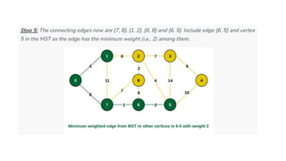
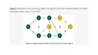
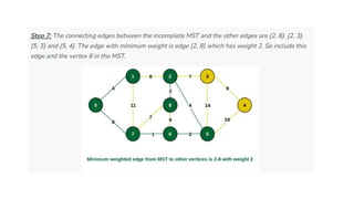
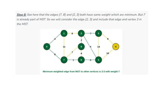
BER2013 – Algorithm Design & Analysis
CLO4:Apply greedy and dynamic algorithm in
programing-based problem.
General characteristics of Greedy algorithms •
Graphs MST - Kruskal's and Prims's algorithms •
Graphs: shortest paths • Knapsack problem
Greedy Algorithms
• The general structure of a greedy algorithm can be summarized in the
following steps:
1.Identify the problem as an optimization problem where we need to find
the best solution among a set of possible solutions.
2.Determine the set of feasible solutions for the problem.
3.Identify the optimal substructure of the problem, meaning that the
optimal solution to the problem can be constructed from the optimal
solutions of its subproblems.
4.Develop a greedy strategy to construct a feasible solution step by step,
making the locally optimal choice at each step.
Prove the correctness of the algorithm by showing that the locally
optimal choices at each step lead to a globally optimal solution.
Greedy Algorithms
• All greedy algorithms follow a basic structure:
1.declare an empty result = 0.
2.We make a greedy choice to select, If the choice is feasible add it to the final result.
3.return the result.
Greedy Algorithms
• Why choose Greedy Approach:
The greedy approach has a few tradeoffs, which may make it suitable for
optimization. One prominent reason is to achieve the most feasible
solution immediately. In the activity selection problem. if more activities
can be done before finishing the current activity, these activities can be
performed within the same time. Another reason is to divide a problem
recursively based on a condition, with no need to combine all the
solutions. In the activity selection problem, the “recursive division” step is
achieved by scanning a list of items only once and considering certain
activities.
Greedy Algorithms
• Greedy choice property:
This property says that the globally optimal solution can be
obtained by making a locally optimal solution (Greedy). The
choice made by a Greedy algorithm may depend on earlier
choices but not on the future. It iteratively makes one Greedy
choice after another and reduces the given problem to a smaller
one.
Optimal substructure:
A problem exhibits optimal substructure if an optimal solution to
the problem contains optimal solutions to the subproblems. That
means we can solve subproblems and build up the solutions to
solve larger problems.
Greedy Algorithms
• Characteristic components of greedy algorithm:
1.The feasible solution: A subset of given inputs that satisfies all specified constraints of a
problem is known as a “feasible solution”.
2.Optimal solution: The feasible solution that achieves the desired extremum is called an
“optimal solution”. In other words, the feasible solution that either minimizes or maximizes
the objective function specified in a problem is known as an “optimal solution”.
3.Feasibility check: It investigates whether the selected input fulfils all constraints mentioned
in a problem or not. If it fulfils all the constraints then it is added to a set of feasible
solutions; otherwise, it is rejected.
4.Optimality check: It investigates whether a selected input produces either a minimum or
maximum value of the objective function by fulfilling all the specified constraints. If an
element in a solution set produces the desired extremum, then it is added to a sel of
optimal solutions.
5.Optimal substructure property: The globally optimal solution to a problem includes the
optimal sub solutions within it.
6.Greedy choice property: The globally optimal solution is assembled by selecting locally
optimal choices. The greedy approach applies some locally optimal criteria to obtain a
partial solution that seems to be the best at that moment and then find out the solution for
the remaining sub-problem.
Greedy Algorithms
Applications of Greedy Algorithms:
• Finding an optimal solution (Activity selection, Fractional Knapsack, Job Sequencing, Huffman Coding).
• Finding close to the optimal solution for NP-Hard problems like TSP.
• Network design: Greedy algorithms can be used to design efficient networks, such as minimum spanning
trees, shortest paths, and maximum flow networks. These algorithms can be applied to a wide range of
network design problems, such as routing, resource allocation, and capacity planning.
• Machine learning: Greedy algorithms can be used in machine learning applications, such as feature selection,
clustering, and classification. In feature selection, greedy algorithms are used to select a subset of features
that are most relevant to a given problem. In clustering and classification, greedy algorithms can be used to
optimize the selection of clusters or classes.
• Image processing: Greedy algorithms can be used to solve a wide range of image processing problems, such
as image compression, denoising, and segmentation. For example, Huffman coding is a greedy algorithm that
can be used to compress digital images by efficiently encoding the most frequent pixels.
• Combinatorial optimization: Greedy algorithms can be used to solve combinatorial optimization problems, such
as the traveling salesman problem, graph coloring, and scheduling. Although these problems are typically NP-
hard, greedy algorithms can often provide close-to-optimal solutions that are practical and efficient.
• Game theory: Greedy algorithms can be used in game theory applications, such as finding the optimal strategy
for games like chess or poker. In these applications, greedy algorithms can be used to identify the most
promising moves or actions at each turn, based on the current state of the game.
• Financial optimization: Greedy algorithms can be used in financial applications, such as portfolio optimization
and risk management. In portfolio optimization, greedy algorithms can be used to select a subset of assets that
are most likely to provide the best return on investment, based on historical data and current market trends.
Greedy Algorithms
• Standard Greedy Algorithms :
• Prim’s Algorithm
• Kruskal’s Algorithm
• Dijkstra’s Algorithm
Prims algorithm
• Prim's algorithm was invented in 1930 by the Czech mathematician Vojtěch
Jarník.
• The algorithm was then rediscovered by Robert C. Prim in 1957, and also
rediscovered by Edsger W. Dijkstra in 1959. Therefore, the algorithm is also
sometimes called "Jarník's algorithm", or the "Prim-Jarník algorithm".
Prims algorithm
• The MST found by Prim's algorithm is the collection of edges in a
graph, that connects all vertices, with a minimum sum of edge
weights.
• Prim's algorithm finds the MST by first including a random vertex
to the MST. The algorithm then finds the vertex with the lowest
edge weight from the current MST, and includes that to the MST.
Prim's algorithm keeps doing this until all nodes are included in
the MST.
• Prim's algorithm is greedy, and has a straightforward way to
create a minimum spanning tree.
• For Prim's algorithm to work, all the nodes must be connected.
To find the MST's in an unconnected graph, Kruskal's
algorithm can be used instead. You can read about Kruskal's
algorithm on the next page.
Prims algorithm
• Step 1: Determine an arbitrary vertex as the starting vertex of the MST.
Step 2: Follow steps 3 to 5 till there are vertices that are not included in
the MST (known as fringe vertex).
Step 3: Find edges connecting any tree vertex with the fringe vertices.
Step 4: Find the minimum among these edges.
Step 5: Add the chosen edge to the MST if it does not form any cycle.
Step 6: Return the MST and exit
Consider the following graph as an example for which we
need to find the Minimum Spanning Tree (MST).
Step 1: Firstly, we select an arbitrary vertex that acts as the starting vertex of
the Minimum Spanning Tree. Here we have selected vertex 0 as the starting
vertex.
Step 2: All the edges connecting the incomplete MST and other vertices are the edges {0, 1} and {0,
7}. Between these two the edge with minimum weight is {0, 1}. So include the edge and vertex 1 in the
MST.
Kruskal’s algorithm
• Here we will discuss Kruskal’s algorithm to find the MST of a
given weighted graph.
• In Kruskal’s algorithm, sort all edges of the given graph in
increasing order. Then it keeps on adding new edges and nodes
in the MST if the newly added edge does not form a cycle. It
picks the minimum weighted edge at first and the maximum
weighted edge at last. Thus we can say that it makes a locally
optimal choice in each step in order to find the optimal solution.
Hence this is a Greedy Algorithm.
Kruskal’s algorithm
• How to find MST using Kruskal’s algorithm?
• We start from the edges with the lowest weight and keep adding edges
until we reach our goal.
• The steps for implementing Kruskal's algorithm are as follows:
1.Sort all the edges from low weight to high
2.Take the edge with the lowest weight and add it to the spanning tree. If
adding the edge created a cycle, then reject this edge.
3.Keep adding edges until we reach all vertices.
Kruskal’s algorithm
The graph contains 9 vertices and 14 edges. So, the
minimum spanning tree formed will be having (9 – 1) = 8
edges.
After sorting:
• Step 1: Pick edge 7-6. No cycle is formed, include it.
• Step 2: Pick edge 8-2. No cycle is formed, include it. Step 4: Pick edge 0-1. No cycle is formed, include it.
Step 3: Pick edge 6-5. No cycle is formed, include it.
• Step 5: Pick edge 2-5. No cycle is formed, include it.
• Step 6: Pick edge 8-6. Since including this edge results in the
cycle, discard it. Pick edge 2-3: No cycle is formed, include it.
• Step 7: Pick edge 7-8. Since including this edge
results in the cycle, discard it. Pick edge 0-7. No cycle is formed (for program refer the *.doc sheet)
include it.
• Step 8: Pick edge 1-2. Since including this edge results in the cycle,
discard it. Pick edge 3-4. No cycle is formed, include it.
•
Knapsack Problem
How to term it?
7. Algorithm Design and analysis ppt.pptx

7. Algorithm Design and analysis ppt.pptx

  • 1.
    BER2013 – AlgorithmDesign & Analysis CLO4:Apply greedy and dynamic algorithm in programing-based problem. General characteristics of Greedy algorithms • Graphs MST - Kruskal's and Prims's algorithms • Graphs: shortest paths • Knapsack problem
  • 2.
    Greedy Algorithms • Thegeneral structure of a greedy algorithm can be summarized in the following steps: 1.Identify the problem as an optimization problem where we need to find the best solution among a set of possible solutions. 2.Determine the set of feasible solutions for the problem. 3.Identify the optimal substructure of the problem, meaning that the optimal solution to the problem can be constructed from the optimal solutions of its subproblems. 4.Develop a greedy strategy to construct a feasible solution step by step, making the locally optimal choice at each step. Prove the correctness of the algorithm by showing that the locally optimal choices at each step lead to a globally optimal solution.
  • 3.
    Greedy Algorithms • Allgreedy algorithms follow a basic structure: 1.declare an empty result = 0. 2.We make a greedy choice to select, If the choice is feasible add it to the final result. 3.return the result.
  • 4.
    Greedy Algorithms • Whychoose Greedy Approach: The greedy approach has a few tradeoffs, which may make it suitable for optimization. One prominent reason is to achieve the most feasible solution immediately. In the activity selection problem. if more activities can be done before finishing the current activity, these activities can be performed within the same time. Another reason is to divide a problem recursively based on a condition, with no need to combine all the solutions. In the activity selection problem, the “recursive division” step is achieved by scanning a list of items only once and considering certain activities.
  • 5.
    Greedy Algorithms • Greedychoice property: This property says that the globally optimal solution can be obtained by making a locally optimal solution (Greedy). The choice made by a Greedy algorithm may depend on earlier choices but not on the future. It iteratively makes one Greedy choice after another and reduces the given problem to a smaller one. Optimal substructure: A problem exhibits optimal substructure if an optimal solution to the problem contains optimal solutions to the subproblems. That means we can solve subproblems and build up the solutions to solve larger problems.
  • 6.
    Greedy Algorithms • Characteristiccomponents of greedy algorithm: 1.The feasible solution: A subset of given inputs that satisfies all specified constraints of a problem is known as a “feasible solution”. 2.Optimal solution: The feasible solution that achieves the desired extremum is called an “optimal solution”. In other words, the feasible solution that either minimizes or maximizes the objective function specified in a problem is known as an “optimal solution”. 3.Feasibility check: It investigates whether the selected input fulfils all constraints mentioned in a problem or not. If it fulfils all the constraints then it is added to a set of feasible solutions; otherwise, it is rejected. 4.Optimality check: It investigates whether a selected input produces either a minimum or maximum value of the objective function by fulfilling all the specified constraints. If an element in a solution set produces the desired extremum, then it is added to a sel of optimal solutions. 5.Optimal substructure property: The globally optimal solution to a problem includes the optimal sub solutions within it. 6.Greedy choice property: The globally optimal solution is assembled by selecting locally optimal choices. The greedy approach applies some locally optimal criteria to obtain a partial solution that seems to be the best at that moment and then find out the solution for the remaining sub-problem.
  • 7.
    Greedy Algorithms Applications ofGreedy Algorithms: • Finding an optimal solution (Activity selection, Fractional Knapsack, Job Sequencing, Huffman Coding). • Finding close to the optimal solution for NP-Hard problems like TSP. • Network design: Greedy algorithms can be used to design efficient networks, such as minimum spanning trees, shortest paths, and maximum flow networks. These algorithms can be applied to a wide range of network design problems, such as routing, resource allocation, and capacity planning. • Machine learning: Greedy algorithms can be used in machine learning applications, such as feature selection, clustering, and classification. In feature selection, greedy algorithms are used to select a subset of features that are most relevant to a given problem. In clustering and classification, greedy algorithms can be used to optimize the selection of clusters or classes. • Image processing: Greedy algorithms can be used to solve a wide range of image processing problems, such as image compression, denoising, and segmentation. For example, Huffman coding is a greedy algorithm that can be used to compress digital images by efficiently encoding the most frequent pixels. • Combinatorial optimization: Greedy algorithms can be used to solve combinatorial optimization problems, such as the traveling salesman problem, graph coloring, and scheduling. Although these problems are typically NP- hard, greedy algorithms can often provide close-to-optimal solutions that are practical and efficient. • Game theory: Greedy algorithms can be used in game theory applications, such as finding the optimal strategy for games like chess or poker. In these applications, greedy algorithms can be used to identify the most promising moves or actions at each turn, based on the current state of the game. • Financial optimization: Greedy algorithms can be used in financial applications, such as portfolio optimization and risk management. In portfolio optimization, greedy algorithms can be used to select a subset of assets that are most likely to provide the best return on investment, based on historical data and current market trends.
  • 8.
    Greedy Algorithms • StandardGreedy Algorithms : • Prim’s Algorithm • Kruskal’s Algorithm • Dijkstra’s Algorithm
  • 9.
    Prims algorithm • Prim'salgorithm was invented in 1930 by the Czech mathematician Vojtěch Jarník. • The algorithm was then rediscovered by Robert C. Prim in 1957, and also rediscovered by Edsger W. Dijkstra in 1959. Therefore, the algorithm is also sometimes called "Jarník's algorithm", or the "Prim-Jarník algorithm".
  • 10.
    Prims algorithm • TheMST found by Prim's algorithm is the collection of edges in a graph, that connects all vertices, with a minimum sum of edge weights. • Prim's algorithm finds the MST by first including a random vertex to the MST. The algorithm then finds the vertex with the lowest edge weight from the current MST, and includes that to the MST. Prim's algorithm keeps doing this until all nodes are included in the MST. • Prim's algorithm is greedy, and has a straightforward way to create a minimum spanning tree. • For Prim's algorithm to work, all the nodes must be connected. To find the MST's in an unconnected graph, Kruskal's algorithm can be used instead. You can read about Kruskal's algorithm on the next page.
  • 11.
    Prims algorithm • Step1: Determine an arbitrary vertex as the starting vertex of the MST. Step 2: Follow steps 3 to 5 till there are vertices that are not included in the MST (known as fringe vertex). Step 3: Find edges connecting any tree vertex with the fringe vertices. Step 4: Find the minimum among these edges. Step 5: Add the chosen edge to the MST if it does not form any cycle. Step 6: Return the MST and exit
  • 12.
    Consider the followinggraph as an example for which we need to find the Minimum Spanning Tree (MST).
  • 13.
    Step 1: Firstly,we select an arbitrary vertex that acts as the starting vertex of the Minimum Spanning Tree. Here we have selected vertex 0 as the starting vertex.
  • 14.
    Step 2: Allthe edges connecting the incomplete MST and other vertices are the edges {0, 1} and {0, 7}. Between these two the edge with minimum weight is {0, 1}. So include the edge and vertex 1 in the MST.
  • 24.
    Kruskal’s algorithm • Herewe will discuss Kruskal’s algorithm to find the MST of a given weighted graph. • In Kruskal’s algorithm, sort all edges of the given graph in increasing order. Then it keeps on adding new edges and nodes in the MST if the newly added edge does not form a cycle. It picks the minimum weighted edge at first and the maximum weighted edge at last. Thus we can say that it makes a locally optimal choice in each step in order to find the optimal solution. Hence this is a Greedy Algorithm.
  • 25.
    Kruskal’s algorithm • Howto find MST using Kruskal’s algorithm? • We start from the edges with the lowest weight and keep adding edges until we reach our goal. • The steps for implementing Kruskal's algorithm are as follows: 1.Sort all the edges from low weight to high 2.Take the edge with the lowest weight and add it to the spanning tree. If adding the edge created a cycle, then reject this edge. 3.Keep adding edges until we reach all vertices.
  • 26.
    Kruskal’s algorithm The graphcontains 9 vertices and 14 edges. So, the minimum spanning tree formed will be having (9 – 1) = 8 edges. After sorting:
  • 27.
    • Step 1:Pick edge 7-6. No cycle is formed, include it. • Step 2: Pick edge 8-2. No cycle is formed, include it. Step 4: Pick edge 0-1. No cycle is formed, include it. Step 3: Pick edge 6-5. No cycle is formed, include it.
  • 28.
    • Step 5:Pick edge 2-5. No cycle is formed, include it. • Step 6: Pick edge 8-6. Since including this edge results in the cycle, discard it. Pick edge 2-3: No cycle is formed, include it.
  • 29.
    • Step 7:Pick edge 7-8. Since including this edge results in the cycle, discard it. Pick edge 0-7. No cycle is formed (for program refer the *.doc sheet) include it. • Step 8: Pick edge 1-2. Since including this edge results in the cycle, discard it. Pick edge 3-4. No cycle is formed, include it. •
  • 30.
  • 31.