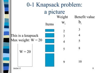
Downloaded 185 times


![04/04/17 5
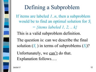
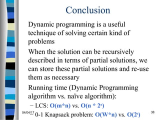
Review: Longest Common
Subsequence (LCS) continued
Define Xi, Yj to be prefixes of X and Y of
length i and j; m = |X|, n = |Y|
We store the length of LCS(Xi, Yj) in c[i,j]
Trivial cases: LCS(X0 , Yj ) and LCS(Xi, Y0)
is empty (so c[0,j] = c[i,0] = 0 )
Recursive formula for c[i,j]:
−−
=+−−
=
otherwise]),1[],1,[max(
],[][if1]1,1[
],[
jicjic
jyixjic
jic
c[m,n] is the final solution](https://image.slidesharecdn.com/0-1knapsack-170404165014/85/0-1-knapsack-5-320.jpg)
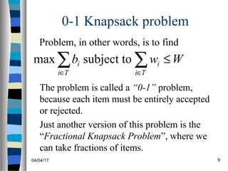
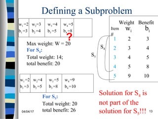
![04/04/17 6
Review: Longest Common
Subsequence (LCS)
After we have filled the array c[ ], we can
use this data to find the characters that
constitute the Longest Common
Subsequence
Algorithm runs in O(m*n), which is much
better than the brute-force algorithm: O(n
2m
)](https://image.slidesharecdn.com/0-1knapsack-170404165014/85/0-1-knapsack-6-320.jpg)
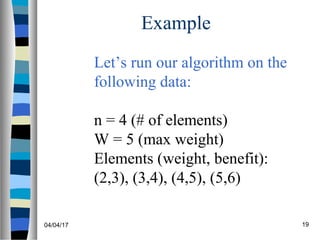
![04/04/17 14
Defining a Subproblem
(continued)
As we have seen, the solution for S4 is not
part of the solution for S5
So our definition of a subproblem is flawed
and we need another one!
Let’s add another parameter: w, which will
represent the exact weight for each subset
of items
The subproblem then will be to compute
B[k,w]](https://image.slidesharecdn.com/0-1knapsack-170404165014/85/0-1-knapsack-14-320.jpg)
![04/04/17 15
Recursive Formula for
subproblems
It means, that the best subset of Sk that has
total weight w is one of the two:
1) the best subset of Sk-1 that has total weight
w, or
2) the best subset of Sk-1 that has total weight
w-wk plus the item k
+−−−
>−
=
else}],1[],,1[max{
if],1[
],[
kk
k
bwwkBwkB
wwwkB
wkB
Recursive formula for subproblems:](https://image.slidesharecdn.com/0-1knapsack-170404165014/85/0-1-knapsack-15-320.jpg)
![04/04/17 16
Recursive Formula
The best subset of Sk that has the total
weight w, either contains item k or not.
First case: wk>w. Item k can’t be part of the
solution, since if it was, the total weight
would be > w, which is unacceptable
Second case: wk <=w. Then the item k can
be in the solution, and we choose the case
with greater value
+−−−
>−
=
else}],1[],,1[max{
if],1[
],[
kk
k
bwwkBwkB
wwwkB
wkB](https://image.slidesharecdn.com/0-1knapsack-170404165014/85/0-1-knapsack-16-320.jpg)
![04/04/17 17
0-1 Knapsack Algorithm
for w = 0 to W
B[0,w] = 0
for i = 0 to n
B[i,0] = 0
for w = 0 to W
if wi <= w // item i can be part of the solution
if bi + B[i-1,w-wi] > B[i-1,w]
B[i,w] = bi + B[i-1,w- wi]
else
B[i,w] = B[i-1,w]
else B[i,w] = B[i-1,w] // wi > w](https://image.slidesharecdn.com/0-1knapsack-170404165014/85/0-1-knapsack-17-320.jpg)
![04/04/17 18
Running time
for w = 0 to W
B[0,w] = 0
for i = 0 to n
B[i,0] = 0
for w = 0 to W
< the rest of the code >
What is the running time of this
algorithm?
O(W)
O(W)
Repeat n times
O(n*W)
Remember that the brute-force algorithm
takes O(2n
)](https://image.slidesharecdn.com/0-1knapsack-170404165014/85/0-1-knapsack-18-320.jpg)
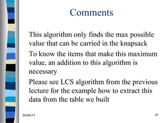
![04/04/17 20
Example (2)
for w = 0 to W
B[0,w] = 0
0
0
0
0
0
0
W
0
1
2
3
4
5
i 0 1 2 3
4](https://image.slidesharecdn.com/0-1knapsack-170404165014/85/0-1-knapsack-20-320.jpg)
![04/04/17 21
Example (3)
for i = 0 to n
B[i,0] = 0
0
0
0
0
0
0
W
0
1
2
3
4
5
i 0 1 2 3
0 0 0 0
4](https://image.slidesharecdn.com/0-1knapsack-170404165014/85/0-1-knapsack-21-320.jpg)
![04/04/17 22
Example (4)
if wi <= w // item i can be part of the solution
if bi + B[i-1,w-wi] > B[i-1,w]
B[i,w] = bi + B[i-1,w- wi]
else
B[i,w] = B[i-1,w]
else B[i,w] = B[i-1,w] // wi > w
0
0
0
0
0
0
W
0
1
2
3
4
5
i 0 1 2 3
0 0 0 0
i=1
bi=3
wi=2
w=1
w-wi =-1
Items:
1: (2,3)
2: (3,4)
3: (4,5)
4: (5,6)
4
0](https://image.slidesharecdn.com/0-1knapsack-170404165014/85/0-1-knapsack-22-320.jpg)
![04/04/17 23
Example (5)
if wi <= w // item i can be part of the solution
if bi + B[i-1,w-wi] > B[i-1,w]
B[i,w] = bi + B[i-1,w- wi]
else
B[i,w] = B[i-1,w]
else B[i,w] = B[i-1,w] // wi > w
0
0
0
0
0
0
W
0
1
2
3
4
5
i 0 1 2 3
0 0 0 0
i=1
bi=3
wi=2
w=2
w-wi =0
Items:
1: (2,3)
2: (3,4)
3: (4,5)
4: (5,6)
4
0
3](https://image.slidesharecdn.com/0-1knapsack-170404165014/85/0-1-knapsack-23-320.jpg)
![04/04/17 24
Example (6)
if wi <= w // item i can be part of the solution
if bi + B[i-1,w-wi] > B[i-1,w]
B[i,w] = bi + B[i-1,w- wi]
else
B[i,w] = B[i-1,w]
else B[i,w] = B[i-1,w] // wi > w
0
0
0
0
0
0
W
0
1
2
3
4
5
i 0 1 2 3
0 0 0 0
i=1
bi=3
wi=2
w=3
w-wi=1
Items:
1: (2,3)
2: (3,4)
3: (4,5)
4: (5,6)
4
0
3
3](https://image.slidesharecdn.com/0-1knapsack-170404165014/85/0-1-knapsack-24-320.jpg)
![04/04/17 25
Example (7)
if wi <= w // item i can be part of the solution
if bi + B[i-1,w-wi] > B[i-1,w]
B[i,w] = bi + B[i-1,w- wi]
else
B[i,w] = B[i-1,w]
else B[i,w] = B[i-1,w] // wi > w
0
0
0
0
0
0
W
0
1
2
3
4
5
i 0 1 2 3
0 0 0 0
i=1
bi=3
wi=2
w=4
w-wi=2
Items:
1: (2,3)
2: (3,4)
3: (4,5)
4: (5,6)
4
0
3
3
3](https://image.slidesharecdn.com/0-1knapsack-170404165014/85/0-1-knapsack-25-320.jpg)
![04/04/17 26
Example (8)
if wi <= w // item i can be part of the solution
if bi + B[i-1,w-wi] > B[i-1,w]
B[i,w] = bi + B[i-1,w- wi]
else
B[i,w] = B[i-1,w]
else B[i,w] = B[i-1,w] // wi > w
0
0
0
0
0
0
W
0
1
2
3
4
5
i 0 1 2 3
0 0 0 0
i=1
bi=3
wi=2
w=5
w-wi=2
Items:
1: (2,3)
2: (3,4)
3: (4,5)
4: (5,6)
4
0
3
3
3
3](https://image.slidesharecdn.com/0-1knapsack-170404165014/85/0-1-knapsack-26-320.jpg)
![04/04/17 27
Example (9)
if wi <= w // item i can be part of the solution
if bi + B[i-1,w-wi] > B[i-1,w]
B[i,w] = bi + B[i-1,w- wi]
else
B[i,w] = B[i-1,w]
else B[i,w] = B[i-1,w] // wi > w
0
0
0
0
0
0
W
0
1
2
3
4
5
i 0 1 2 3
0 0 0 0
i=2
bi=4
wi=3
w=1
w-wi=-2
Items:
1: (2,3)
2: (3,4)
3: (4,5)
4: (5,6)
4
0
3
3
3
3
0](https://image.slidesharecdn.com/0-1knapsack-170404165014/85/0-1-knapsack-27-320.jpg)
![04/04/17 28
Example (10)
if wi <= w // item i can be part of the solution
if bi + B[i-1,w-wi] > B[i-1,w]
B[i,w] = bi + B[i-1,w- wi]
else
B[i,w] = B[i-1,w]
else B[i,w] = B[i-1,w] // wi > w
0
0
0
0
0
0
W
0
1
2
3
4
5
i 0 1 2 3
0 0 0 0
i=2
bi=4
wi=3
w=2
w-wi=-1
Items:
1: (2,3)
2: (3,4)
3: (4,5)
4: (5,6)
4
0
3
3
3
3
0
3](https://image.slidesharecdn.com/0-1knapsack-170404165014/85/0-1-knapsack-28-320.jpg)
![04/04/17 29
Example (11)
if wi <= w // item i can be part of the solution
if bi + B[i-1,w-wi] > B[i-1,w]
B[i,w] = bi + B[i-1,w- wi]
else
B[i,w] = B[i-1,w]
else B[i,w] = B[i-1,w] // wi > w
0
0
0
0
0
0
W
0
1
2
3
4
5
i 0 1 2 3
0 0 0 0
i=2
bi=4
wi=3
w=3
w-wi=0
Items:
1: (2,3)
2: (3,4)
3: (4,5)
4: (5,6)
4
0
3
3
3
3
0
3
4](https://image.slidesharecdn.com/0-1knapsack-170404165014/85/0-1-knapsack-29-320.jpg)
![04/04/17 30
Example (12)
if wi <= w // item i can be part of the solution
if bi + B[i-1,w-wi] > B[i-1,w]
B[i,w] = bi + B[i-1,w- wi]
else
B[i,w] = B[i-1,w]
else B[i,w] = B[i-1,w] // wi > w
0
0
0
0
0
0
W
0
1
2
3
4
5
i 0 1 2 3
0 0 0 0
i=2
bi=4
wi=3
w=4
w-wi=1
Items:
1: (2,3)
2: (3,4)
3: (4,5)
4: (5,6)
4
0
3
3
3
3
0
3
4
4](https://image.slidesharecdn.com/0-1knapsack-170404165014/85/0-1-knapsack-30-320.jpg)
![04/04/17 31
Example (13)
if wi <= w // item i can be part of the solution
if bi + B[i-1,w-wi] > B[i-1,w]
B[i,w] = bi + B[i-1,w- wi]
else
B[i,w] = B[i-1,w]
else B[i,w] = B[i-1,w] // wi > w
0
0
0
0
0
0
W
0
1
2
3
4
5
i 0 1 2 3
0 0 0 0
i=2
bi=4
wi=3
w=5
w-wi=2
Items:
1: (2,3)
2: (3,4)
3: (4,5)
4: (5,6)
4
0
3
3
3
3
0
3
4
4
7](https://image.slidesharecdn.com/0-1knapsack-170404165014/85/0-1-knapsack-31-320.jpg)
![04/04/17 32
Example (14)
if wi <= w // item i can be part of the solution
if bi + B[i-1,w-wi] > B[i-1,w]
B[i,w] = bi + B[i-1,w- wi]
else
B[i,w] = B[i-1,w]
else B[i,w] = B[i-1,w] // wi > w
0
0
0
0
0
0
W
0
1
2
3
4
5
i 0 1 2 3
0 0 0 0
i=3
bi=5
wi=4
w=1..3
Items:
1: (2,3)
2: (3,4)
3: (4,5)
4: (5,6)
4
0
3
3
3
3
00
3
4
4
7
0
3
4](https://image.slidesharecdn.com/0-1knapsack-170404165014/85/0-1-knapsack-32-320.jpg)
![04/04/17 33
Example (15)
if wi <= w // item i can be part of the solution
if bi + B[i-1,w-wi] > B[i-1,w]
B[i,w] = bi + B[i-1,w- wi]
else
B[i,w] = B[i-1,w]
else B[i,w] = B[i-1,w] // wi > w
0
0
0
0
0
0
W
0
1
2
3
4
5
i 0 1 2 3
0 0 0 0
i=3
bi=5
wi=4
w=4
w- wi=0
Items:
1: (2,3)
2: (3,4)
3: (4,5)
4: (5,6)
4
0 00
3
4
4
7
0
3
4
5
3
3
3
3](https://image.slidesharecdn.com/0-1knapsack-170404165014/85/0-1-knapsack-33-320.jpg)
![04/04/17 34
Example (15)
if wi <= w // item i can be part of the solution
if bi + B[i-1,w-wi] > B[i-1,w]
B[i,w] = bi + B[i-1,w- wi]
else
B[i,w] = B[i-1,w]
else B[i,w] = B[i-1,w] // wi > w
0
0
0
0
0
0
W
0
1
2
3
4
5
i 0 1 2 3
0 0 0 0
i=3
bi=5
wi=4
w=5
w- wi=1
Items:
1: (2,3)
2: (3,4)
3: (4,5)
4: (5,6)
4
0 00
3
4
4
7
0
3
4
5
7
3
3
3
3](https://image.slidesharecdn.com/0-1knapsack-170404165014/85/0-1-knapsack-34-320.jpg)
![04/04/17 35
Example (16)
if wi <= w // item i can be part of the solution
if bi + B[i-1,w-wi] > B[i-1,w]
B[i,w] = bi + B[i-1,w- wi]
else
B[i,w] = B[i-1,w]
else B[i,w] = B[i-1,w] // wi > w
0
0
0
0
0
0
W
0
1
2
3
4
5
i 0 1 2 3
0 0 0 0
i=3
bi=5
wi=4
w=1..4
Items:
1: (2,3)
2: (3,4)
3: (4,5)
4: (5,6)
4
0 00
3
4
4
7
0
3
4
5
7
0
3
4
5
3
3
3
3](https://image.slidesharecdn.com/0-1knapsack-170404165014/85/0-1-knapsack-35-320.jpg)
![04/04/17 36
Example (17)
if wi <= w // item i can be part of the solution
if bi + B[i-1,w-wi] > B[i-1,w]
B[i,w] = bi + B[i-1,w- wi]
else
B[i,w] = B[i-1,w]
else B[i,w] = B[i-1,w] // wi > w
0
0
0
0
0
0
W
0
1
2
3
4
5
i 0 1 2 3
0 0 0 0
i=3
bi=5
wi=4
w=5
Items:
1: (2,3)
2: (3,4)
3: (4,5)
4: (5,6)
4
0 00
3
4
4
7
0
3
4
5
7
0
3
4
5
7
3
3
3
3](https://image.slidesharecdn.com/0-1knapsack-170404165014/85/0-1-knapsack-36-320.jpg)


The document discusses the 0-1 knapsack problem and how it can be solved using dynamic programming. It first defines the 0-1 knapsack problem and provides an example. It then explains how a brute force solution would work in exponential time. Next, it describes how to define the problem as subproblems and derive a recursive formula to solve the subproblems in a bottom-up manner using dynamic programming. This builds up the solutions in a table and solves the problem in polynomial time. Finally, it walks through an example applying the dynamic programming algorithm to a sample problem instance.