Download to read offline
![> PAPER IDENTIFICATION NUMBER TBD< 7
D. MATH EXAMPLE 4: RODDY EXAMPLE 10.1 page
304
The author interest is to estimate BER for binary polar
transmission; given 𝐸 𝑏 = 1𝐸 − 06 & 𝑁 = 1𝐸 − 07. This
example is surprisingly confusing as simple as it can look. As
known,
𝐸 𝑏
𝑁
=
1𝐸 − 06
1𝐸 − 07
= 10
Now, the author uses erf instead of erfc. The relationship
between these two functions is that their sum =1. That is,
erf(𝑥) + 𝑒𝑟𝑓𝑐(𝑥) = 1. (12)
Now, in order to properly solve the problem, you must
know that for polar signaling the correct formulas are the ones
we used with the above example:
𝑃𝑒 = 𝑄 (√
2𝐸 𝑏
𝑁
) (13)
Solving,
𝑃𝑒 = 𝑄 (√
2𝐸 𝑏
𝑁
) = 𝑄 (√(2 ∗ 10)) =
𝑄(√20) 𝑄(4.472135955)3.872108𝐸 − 06
It is important to understand that 𝑧 = √20 4.472135955
here; thus, 𝑥 =
𝑧
√2
=
√20
√2
= √103.16227766
Using erfc,
𝑃𝑒 = 𝑒𝑟𝑓𝑐(𝑥) =
1 − 𝐺𝐴𝑀𝑀𝐴. 𝐷𝐼𝑆𝑇(𝑥2
, 0.5,1,1)
2
1 − 𝐺𝐴𝑀𝑀𝐴. 𝐷𝐼𝑆𝑇(3.162277662
, 0.5,1,1)
2
1 − 𝐺𝐴𝑀𝑀𝐴. 𝐷𝐼𝑆𝑇(𝟏𝟎, 0.5,1,1)
2
3.872108𝐸 − 06
The author’s solution using a graphical approach is
surprisingly precise, it gives 𝑃𝑒 = 3.9𝐸 − 06.
And again, the Gamma approach is the easier and
straightforward methodology to find the result.
A student learning from different texts could get very
confused as to what value to input in which function in order
to correctly estimate the BER. This text directs the student to
look for erf(√10) erf(3.16227766). There are no details on
how to do this.
IV. CONCLUSION
It could be appreciated that using examples from three
different authors in texts with different topics the easier way to
avoid confusions and get the correct results with the least
effort was to use the proposed Excel Gamma function.
It is a mistake not to explain in detail the use of the Q(z)
and ercf(x) functions in most communication courses as it is
looked as an easy task not worthy of the time. This paper
illustrates the correct way to code with Excel in order to
always obtain the correct result.
V. APPENDIX
Appendices not needed in this work.
REFERENCES
[1] B.P. Lathi Modern Digital and Analog Communications
Systems 3rd
Ed., Oxford University Press NY, 1998.
[2] T. Pratt, C. W. Bostian & J. E. Allnut Satellite
Communications 2nd
Ed. John Wiley & Sons, MA,
2003.
[3] D. Roddy Satellite Communications 4th
Ed. Mc-Graw
Hill, NY 2006.
XXXXXXXXX.](https://image.slidesharecdn.com/paperrevcatolica2-200112200239/85/Understanding-the-Differences-between-the-erfc-x-and-the-Q-z-functions-A-Simple-Approach-using-Excel-7-320.jpg)

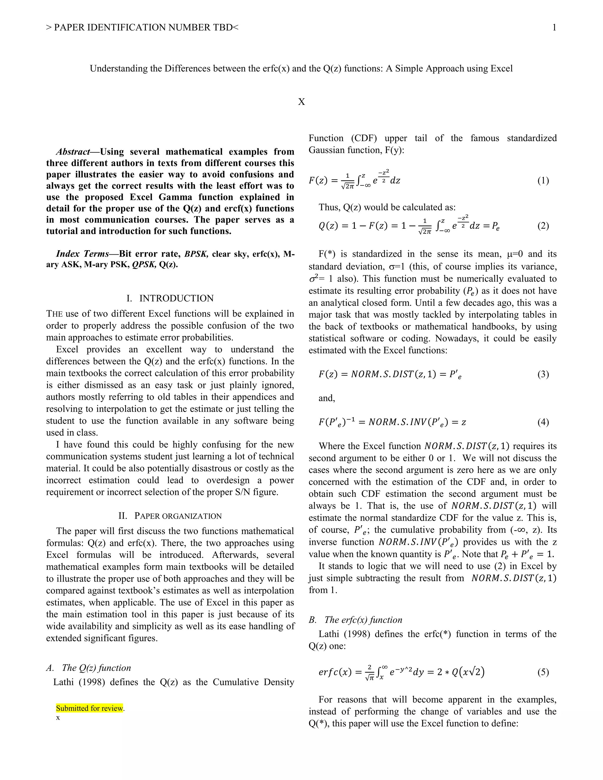
The paper presents a tutorial on using Excel functions q(z) and erfc(x) to accurately estimate error probabilities in communication systems, addressing confusions often faced by students. It emphasizes the advantages of using Excel for these calculations over traditional methods, providing several mathematical examples to illustrate the proper application of these functions. By comparing results from examples in existing textbooks, the paper highlights the effectiveness of the proposed methods in achieving accurate estimations.


![Week7 Quiz Help 2009[1]](https://cdn.slidesharecdn.com/ss_thumbnails/week7quizhelp20091-091012152329-phpapp02-thumbnail.jpg?width=640&height=640&fit=bounds)