1) The document discusses dynamics modeling for robotic manipulators using the Denavit-Hartenberg representation and Lagrangian mechanics. It describes using the Euler-Lagrange method to derive equations of motion for robotic links by computing kinetic and potential energy terms. 2) As an example, dynamics equations are derived for a simple 1 degree-of-freedom robotic arm. Kinetic and potential energy expressions are written and the Lagrangian is computed to obtain the equation of motion. 3) State-space modeling basics are reviewed using the example of a damped spring-mass system, showing how to write the system dynamics as state-space matrices to evaluate responses like step response.

1. Dynamics for Robotic Manipulators
Notes for the Robotics Lecture
Dr. Marco Antonio P´erez-Cisneros
marcopc@cucei.udg.mx
Electronics and Computer Science Division
Exact Sciences and Engineering Campus, CUCEI
Universidad de Guadalajara
&
Control Systems Centre
UMIST, Manchester, UK
v2.0 November 2005

2. Chapter 1
Introduction
The study has discussed about manipulators being conformed by a number of
links within a mechanic linkage bounded by joints. So far, two basic types of joints
have been described: revolute and prismatic. It is possible to use the Denavit-
Hertenberg representation to model each of the links in such a way that the whole
robotic plant can be simply represented by a Kinematic description. In the DH
standard, each link is assumed to have its z axis pointing to the rotation axis or
to the prismatic direction of movement. The displacement required between two
frames previosly assigned to the two joints in the same link is always calculated
in the direction pointed by the x or z axis. Rotation adjustments between two
rotation axis (or displacement axis in case of prismatic joints) are performed over
the x axis exclusively.
In standard conditions, the Kinematic model is normally expressed in terms
of the vector q which groups the so-called generalized coordinates q1, q1, . . . qn.
However such arrangement also exhibits dynamic response to the forces and
torques exerted over the whole linkage. For instance the gravity forces and the
torques applied to joints by means of actuators. In this case vector q is used to
represent the motion of every particle belonging to a link in terms of only one
coordinate.
Assuming that the distance between a given pair of particles belonging to one
link is fixed throughout the movements, it is possible to use only six coordinates
to completely represent the position and orientation of each particle in the robotic
link.
It is merely at this point, that the Dynamic analysis comes at hand. It
describes the behavior of each robots link in terms of the time rate of change
with respect to the joint torques exerted by the actuators. This assumption refers
to a set of differential equations, called the equations of motion that dictate the
dynamic response according the time evolution.
Two methods can be used to derive the Dynamics equations of motion. First,
the Newton-Euler method treaters each individual link of the robot by writing
down equations to describe linear and angular motions.
1

3. Since each link is coupled to others, contact forces and torques also appear in
the equations to describe neighboring links. In the so called forward-backwards
recursive cycle, the coupling terms are determined and the manipulator can be
therefore be described as a whole. Unfortunately the analysis gets very compli-
cated if the number of links operating the arm is increased.
Second comes the Euler-Lagrange method which is based on the algorithm of
virtual displacements and energy dissipation. This is a set of infinitesimal shifts
under the known constraints of the robotic chain which result from a difference
between the kinetic and potential energy.
For simplicity in this chapter, only the Euler-Lagrange methods is further con-
sidered. An interested reader may consult the remarkable study of the Newton-
Euler method presented by Spong in [1].
2

4. Chapter 2
Lagrange´s motion equations
Considering a manipulator conformed by n links, the total energy ε contained by
an n-DOF system is equal to the total sum of kinetics κ and potential υ energy
as follows:
ε(q(t), ˙q(t)) = κ(q(t), ˙q(t)) + υ(q(t)) (2.1)
with the generalized coordinates vector q = [q1, q1, . . . qn]T
. Following the clear
exposition in [2], the Lagrangian L of a manipulator of n-DOF is therefore the
difference between the kinetic κ and potential υ energy yielding
L(q(t), ˙q(t)) = κ(q(t), ˙q(t)) − υ(q(t)) (2.2)
It is assumed that the potential energy is generated by the conservative forces
such as gravity and spring-like effects. The complete Lagrangian is thus defined
as follows
d
dt
∂L(q(t), ˙q(t))
∂ ˙qi
−
∂L(q(t), ˙q(t))
∂qi
= τi i = 1, . . . , n (2.3)
with τi being the forces and the torques externally exerted by actuators over each
link. Also the non-conservative forces produced by friction, motion opposition
and all those which depend upon time or speed.
Notice that there will be as many scalar equations as the number of the DOF.
In order to build the dynamical model of a given manipulator, each of the
terms in Equation 2.3 needs to be computed by following the steps below:
1. Kinetic energy computation κ(q(t), ˙q(t))
2. Potential energy υ(q(t))
3. Building the Lagrangian operator L(q(t), ˙q(t))
4. Developing Lagrange’s equation of motion (Eq. 2.3).
3

5. 2.0.1 Example 1
Let’s analyze a very simple example taken from [2]. See Figure 2.1, it has a very
simple robotic arm, with only one DOF since angle ϕ is constant. The robot has
only one link with two sections of longitude l1 and l2. For simplicity, the mass of
each link is supposed to be punctual and located at the end of the link.
Figure 2.1: A simple robotic plant for modeling its Dynamics
The robot has only rotation movements around its base. So the only DOF is
thus named as q(t) = q1(t).
The kinematic energy κ(q(t), ˙q(t)) is computed as the product of one half of
the inertia1 1
2
m2l2
2cos2
(ϕ) and the angular velocity ˙q2
as follows:
κ(q(t), ˙q(t)) =
1
2
m2l2
2cos2
(ϕ) ˙q2
(2.4)
The potential energy can be calculated by considering the plane x0 − y0 with
zero energy. So, it yields
υ(q(t)) = m1l1g + m2[l1 + l2 sin(ϕ)]g (2.5)
with g representing the gravity vector g = [0, 0, g]. In fact, for this specific
example, the potential energy is a constant since it does not depend on the angle
value q1. So, finally building the Lagrange operator yields
L(q(t), ˙q(t)) =
m2
2
l2
2cos2
(ϕ) ˙q2
− m1l1g − m2[l1 + l2 sin(ϕ)]g (2.6)
1
Recall Inertia is the property of one element to store kinetic energy derived from a rotation
movement. For instance, in circular movements the inertia is given by I = 1
2 Mr2
4

6. from it is very easy to obtain
∂L
∂ ˙qi
= m2l2
2cos2
(ϕ) ˙q
d
dt
∂L
∂ ˙qi
= m2l2
2cos2
(ϕ)¨q
∂L
∂qi
= 0
(2.7)
and therefore Equation 2.3 results in
m2l2
2cos2
(ϕ)¨q = τ (2.8)
with τ being the torque applied to joint one. Although very simple, after ap-
plying the second Newton’s law, it yields a non-autonomous second-order linear
differential equation.
So this equation can also be expressed using state-space variables yielding
d
dt
q
˙q
=
˙q
1
m2l2
2cos2(ϕ)
τ(t) (2.9)
2.0.2 Revisiting State-Space Modelling
In case the concepts of system modeling using state-space variables are not fresh
enough, a quick review of the basic principles is presented below.
m
k
b
p
x0
Figure 2.2: The damp-spring-mass mechanical system.
As main example, recall the typical damp-spring-mass (DSM) mechanical
system [3] shown in Figure 2.2. The input to the system is the force applied to
the mass body which results in a change in the objects position x and considered
as the system output. This system can be understood as an analogy to the serial
connection of one resistor, one inductor and one capacitor. Naming the spring
5

7. constant as k, the damper value as b and the objects mass as m, the equation for
the system’s dynamics can be drawn as follows
m
d2
x
dt2
+ b
dx
dt
+ kx = p (2.10)
writing the expression in a more convinient way considering all the derivatives
are calculated with respect to time, it follows
m¨x + b ˙x + kx = p (2.11)
Clearing the derivative of highest order, it yields
¨x = −
b
m
˙x −
k
m
x +
p
m
(2.12)
It is time to assign a new set of variables to each of the derivative expressions,
following some simple rules:
• Assign as many variables as necessary until n − 1, with n being the highest
derivative order.
• Draw equivalent terms such as x2 = ˙x1
• Substitute the new set of variables in the original expression.
• Build the state-space matrices by grouping the state-variables in only one
state vector x.
So following Equation 2.12, the new set of state-variables and its equivalences
can be drawn as follows:
x1 = x
x2 = ˙x x2 = ˙x1
(2.13)
transforming the expression 2.12 as follows
˙x2 = −
b
m
x2 −
k
m
x1 +
p
m
(2.14)
which easily gives way to the matrix form ˙x = Ax + B.
˙x1
˙x2
=
0 1
− k
m
− b
m
x1
x2
+
0
p
m
(2.15)
and the output has the matrix form y = Cx + D as follows:
y =
1 0
0 1
x1
x2
+
0
0
(2.16)
6

8. 0
5
10
15
To:Out(1)
0 50 100 150 200 250
−0.4
−0.2
0
0.2
0.4
0.6
0.8
1
To:Out(2)
Step Response
Time (sec)
Amplitude
Figure 2.3: Step response of the damp-spring-mass system.
The last expression allows to chose the output of the system according to the
user preference. In this case the output is represented by x1 which is in time the
object’s displacement x.
Matlab comes naturally prepared to evaluate state-space functions. The sys-
tem is easily defined by supplying the values for the four state matrices A, B, C
and D. A simple example is given for the following values of the damp-spring-
mass system: k = 0.1, b = 0.5, p = 1Nw
m
and m = 10kg. Figure 2.3 shows
the output of the step response command in Matlab as detailed in Algorithm 2.1.
7

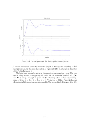
9. Algorithm 2.1 Matlab commands for the step-response of the damp-spring-mass
system expressed by space-state matrices.
1: m=10;
2: k=0.1;
3: b=0.5;
4: p=1;
5: A = [0 1; -k/m -b/m];
6: B = [0; p/m];
7: C=[1 0; 0 1];
8: D = [0; 0];
9: amortigua = ss(A,B,C,D);
10: step(amortigua)
8

10. Bibliography
[1] M. Spong and M. Vidyasagar. Robot Dynamics and Control. John Wiley,
1989. ISBN 047161243X.
[2] R. Kelly and V. Santibanez. Control de Movimiento de Robots Manipuladores.
Control Automatico e Informatica Industrial. Pearson-Prentice Hall, 2003.
[3] Katsuhiko Ogata. Modern Control Engineering. Prentice-Hall, 1997. ISBN
0132273071.
9