This document presents and compares three approximation methods for thin plate spline mappings that reduce the computational complexity from O(p3) to O(m3), where m is a small subset of points p. Method 1 uses only the subset of points to estimate the mapping. Method 2 uses the subset of basis functions with all target values. Method 3 approximates the full matrix using the Nyström method. Experiments on synthetic grids show Method 3 has the lowest error, followed by Method 2, with Method 1 having the highest error. The three methods trade off accuracy, computation time, and the ability to do principal warp analysis.

1. Approximate Thin Plate Spline Mappings
Gianluca Donato1
and Serge Belongie2
1
Digital Persona, Inc., Redwood City, CA 94063
gianlucad@digitalpersona.com
2
U.C. San Diego, La Jolla, CA 92093-0114
sjb@cs.ucsd.edu
Abstract. The thin plate spline (TPS) is an effective tool for modeling
coordinate transformations that has been applied successfully in several
computer vision applications. Unfortunately the solution requires the in-
version of a p×p matrix, where p is the number of points in the data set,
thus making it impractical for large scale applications. As it turns out,
a surprisingly good approximate solution is often possible using only a
small subset of corresponding points. We begin by discussing the obvious
approach of using the subsampled set to estimate a transformation that is
then applied to all the points, and we show the drawbacks of this method.
We then proceed to borrow a technique from the machine learning com-
munity for function approximation using radial basis functions (RBFs)
and adapt it to the task at hand. Using this method, we demonstrate
a significant improvement over the naive method. One drawback of this
method, however, is that is does not allow for principal warp analysis,
a technique for studying shape deformations introduced by Bookstein
based on the eigenvectors of the p × p bending energy matrix. To ad-
dress this, we describe a third approximation method based on a classic
matrix completion technique that allows for principal warp analysis as
a by-product. By means of experiments on real and synthetic data, we
demonstrate the pros and cons of these different approximations so as
to allow the reader to make an informed decision suited to his or her
application.
1 Introduction
The thin plate spline (TPS) is a commonly used basis function for representing
coordinate mappings from R2
to R2
. Bookstein [3] and Davis et al. [5], for exam-
ple, have studied its application to the problem of modeling changes in biological
forms. The thin plate spline is the 2D generalization of the cubic spline. In its
regularized form the TPS model includes the affine model as a special case.
One drawback of the TPS model is that its solution requires the inversion
of a large, dense matrix of size p × p, where p is the number of points in the
data set. Our goal in this paper is to present and compare three approximation
methods that address this computational problem through the use of a subset of
corresponding points. In doing so, we highlight connections to related approaches
in the area of Gaussian RBF networks that are relevant to the TPS mapping
A. Heyden et al. (Eds.): ECCV 2002, LNCS 2352, pp. 21–31, 2002.
c Springer-Verlag Berlin Heidelberg 2002

2. 22 G. Donato and S. Belongie
problem. Finally, we discuss a novel application of the Nystr¨om approximation
[1] to the TPS mapping problem.
Our experimental results suggest that the present work should be particu-
larly useful in applications such as shape matching and correspondence recovery
(e.g. [2,7,4]) as well as in graphics applications such as morphing.
2 Review of Thin Plate Splines
Let vi denote the target function values at locations (xi, yi) in the plane, with
i = 1, 2, . . . , p. In particular, we will set vi equal to the target coordinates
(xi,yi) in turn to obtain one continuous transformation for each coordinate. We
assume that the locations (xi, yi) are all different and are not collinear. The TPS
interpolant f(x, y) minimizes the bending energy
If =
R2
(f2
xx + 2f2
xy + f2
yy)dxdy
and has the form
f(x, y) = a1 + axx + ayy +
p
i=1
wiU ( (xi, yi) − (x, y) )
where U(r) = r2
log r. In order for f(x, y) to have square integrable second
derivatives, we require that
p
i=1
wi = 0 and
p
i=1
wixi =
p
i=1
wiyi = 0 .
Together with the interpolation conditions, f(xi, yi) = vi, this yields a linear
system for the TPS coefficients:
K P
PT
O
w
a
=
v
o
(1)
where Kij = U( (xi, yi) − (xj, yj) ), the ith row of P is (1, xi, yi), O is a 3 × 3
matrix of zeros, o is a 3 × 1 column vector of zeros, w and v are column vectors
formed from wi and vi, respectively, and a is the column vector with elements
a1, ax, ay. We will denote the (p + 3) × (p + 3) matrix of this system by L; as
discussed e.g. in [7], L is nonsingular. If we denote the upper left p × p block of
L−1
by L−1
p , then it can be shown that
If ∝ vT
L−1
p v = wT
Kw .

3. Approximate Thin Plate Spline Mappings 23
When there is noise in the specified values vi, one may wish to relax the exact
interpolation requirement by means of regularization. This is accomplished by
minimizing
H[f] =
n
i=1
(vi − f(xi, yi))2
+ λIf .
The regularization parameter λ, a positive scalar, controls the amount of smooth-
ing; the limiting case of λ = 0 reduces to exact interpolation. As demonstrated
in [9,6], we can solve for the TPS coefficients in the regularized case by replacing
the matrix K by K + λI, where I is the p × p identity matrix.
3 Approximation Techniques
Since inverting L is an O(p3
) operation, solving for the TPS coefficients can be
very expensive when p is large. We will now discuss three different approximation
methods that reduce this computational burden to O(m3
), where m can be as
small as 0.1p. The corresponding savings factors in memory (5x) and processing
time (1000x) thus make TPS methods tractable when p is very large.
In the discussion below we use the following partition of the K matrix:
K =
A B
BT
C
(2)
with A ∈ Rm×m
, B ∈ Rm×n
, and C ∈ Rn×n
. Without loss of generality, we
will assume the p points are labeled in random order, so that the first m points
represent a randomly selected subset.
3.1 Method 1: Simple Subsampling
The simplest approximation technique is to solve for the TPS mapping between
a randomly selected subset of the correspondences. This amounts to using A
in place of K in Equation (1). We can then use the recovered coefficients to
extrapolate the TPS mapping to the remaining points. The result of applying
this approximation to some sample shapes is shown in Figure 1. In this case,
certain parts were not sampled at all, and as a result the mapping in those areas
is poor.
3.2 Method 2: Basis Function Subset
An improved approximation can be obtained by using a subset of the basis
functions with all of the target values. Such an approach appears in [10,6] and
Section 3.1 of [8] for the case of Gaussian RBFs. In the TPS case, we need to
account for the affine terms, which leads to a modified set of linear equations.
Starting from the cost function
R[ ˜w, a] =
1
2
v − ˜K ˜w − Pa 2
+
λ
2
˜wT
A ˜w ,

4. 24 G. Donato and S. Belongie
(a) (b) (c) (d)
(e) (f) (g) (h)
Fig. 1. Thin plate spline (TPS) mapping example. (a,b) Template and target synthetic
fish shapes, each consisting of 98 points. (Correspondences between the two shapes are
known.) (c) TPS mapping of (a) onto (b) using the subset of points indicated by circles
(Method 1). Corresponding points are indicated by connecting line segments. Notice
the quality of the mapping is poor where the samples are sparse. An improved approxi-
mation can be obtained by making use of the full set of target values; this is illustrated
in (d), where we have used Method 2 (discussed in Section 3.2). A similar mapping is
found for the same set of samples using Method 3 (see Section 3.3). In (e-h) we observe
the same behavior for a pair of handwritten digits, where the correspondences (89 in
all) have been found using the method of [2].
we minimize it by setting ∂R/∂ ˜w and ∂R/∂a to zero, which leads to the following
(m + 3) × (m + 3) linear system,
˜KT ˜K + λA ˜KT
P
PT ˜K PT
P
˜w
a
=
˜KT
v
PT
v
(3)
where ˜KT
= [A BT
], ˜w is an m × 1 vector of TPS coefficients, and the rest
of the entries are as before. Thus we seek weights for the reduced set of basis
functions that take into account the full set of p target values contained in v. If
we call ˜P the first m rows of P and ˜I the first m columns of the p × p identity
matrix, then under the assumption ˜PT
˜w = 0, Equation (3) is equivalent to
˜K + λ˜I P
˜PT
O
˜w
a
=
v
o
which corresponds to the regularized version of Equation (1) when using the
subsampled ˜K and ˜PT
in place of K and PT
.
The application of this technique to the fish and digit shapes is shown in
Figure 1(d,h).

5. Approximate Thin Plate Spline Mappings 25
3.3 Method 3: Matrix Approximation
The essence of Method 2 was to use a subset of exact basis functions to approx-
imate a full set of target values. We now consider an approach that uses a full
set of approximate basis functions to approximate the full set of target values.
The approach is based on a technique known as the Nystr¨om method.
The Nystr¨om method provides a means of approximating the eigenvectors
of K without using C. It was originally developed in the late 1920s for the
numerical solution of eigenfunction problems [1] and was recently used in [11]
for fast approximate Gaussian process regression and in [8] (implicitly) to speed
up several machine learning techniques using Gaussian kernels. Implicit to the
Nystr¨om method is the assumption that C can be approximated by BT
A−1
B,
i.e.
ˆK =
A B
BT
BT
A−1
B
(4)
If rank(K) = m and the m rows of the submatrix [A B] are linearly indepen-
dent, then ˆK = K. In general, the quality of the approximation can be expressed
as the norm of the difference C − BT
A−1
B, the Schur complement of K.
Given the m × m diagonalization A = UΛUT
, we can proceed to find the
approximate eigenvectors of K:
ˆK = ˜UΛ ˜UT
, with ˜U =
U
BT
UΛ−1 (5)
Note that in general the columns of ˜U are not orthogonal. To address this, first
define Z = ˜UΛ1/2
so that ˆK = ZZT
. Let QΣQT
denote the diagonalization
of ZT
Z. Then the matrix V = ZQΣ−1/2
contains the leading orthonormalized
eigenvectors of ˆK, i.e. ˆK = V ΣV T
, with V T
V = I.
From the standard formula for the partitioned inverse of L, we have
L−1
=
K−1
+ K−1
PS−1
PT
K−1
−K−1
PS−1
−S−1
PT
K−1
S−1 , S = −PT
K−1
P
and thus
w
a
= L−1 v
o
=
(I + K−1
PS−1
PT
)K−1
v
−S−1
PT
K−1
v
Using the Nystr¨om approximation to K, we have ˆK−1
= V Σ−1
V T
and
ˆw = (I + V Σ−1
V T
P ˆS−1
PT
)V Σ−1
V T
v ,
ˆa = − ˆS−1
PT
V Σ−1
V T
v
with ˆS = −PT
V Σ−1
V T
P, which is 3 × 3. Therefore, by computing matrix-
vector products in the appropriate order, we can obtain estimates to the TPS

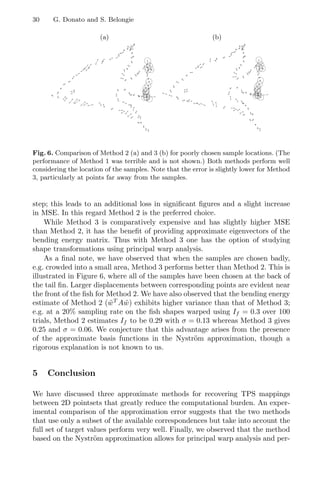
6. 26 G. Donato and S. Belongie
(a) (b) (c)
Fig. 2. Grids used for experimental testing. (a) Reference point set S1: 12 × 12 points
on the interval [0, 128]×[0, 128]. (b,c) Warped point sets S2 and S3 with bending energy
0.3 and 0.8, respectively. To test the quality of the different approximation methods,
we used varying percentages of points to estimate the TPS mapping from S1 to S2 and
from S1 to S3.
coefficients without ever having to invert or store a large p × p matrix. For the
regularized case, one can proceed in the same manner, using
(V ΣV T
+ λI)−1
= V (Σ + λI)−1
V T
.
Finally, the approximate bending energy is given by
wT ˆKw = (V T
w)T
Σ(V T
w)
Note that this bending energy is the average of the energies associated to the x
and y components as in [3].
Let us briefly consider what ˆw represents. The first m components roughly
correspond to the entries in ˜w for Method 2; these in turn correspond to the
columns of ˆK (i.e. ˜K) for which exact information is available. The remaining
entries weight columns of ˆK with (implicitly) filled-in values for all but the
first m entries. In our experiments, we have observed that the latter values of
ˆw are nonzero, which indicates that these approximate basis functions are not
being disregarded. Qualitatively, the approximation quality of methods 2 and 3
are very similar, which is not surprising since they make use of the same basic
information. The pros and cons of these two methods are investigated in the
following section.
4 Experiments
4.1 Synthetic Grid Test
In order to compare the above three approximation methods, we ran a set of
experiments based on warped versions of the cartesian grid shown in Figure 2(a).
The grid consists of 12 × 12 points in a square of dimensions 128 × 128. Call this
set of points S1. Using the technique described in Appendix A, we generated

7. Approximate Thin Plate Spline Mappings 27
5 10 15 20 25 30
0
1
2
3
4
5
6
7
8
Percentage of samples used
MSE
If
=0.3
Method 1
Method 2
Method 3
5 10 15 20 25 30
0
1
2
3
4
5
6
7
8
Percentage of samples used
MSE
If
=0.8
Method 1
Method 2
Method 3
Fig. 3. Comparison of approximation error. Mean squared error in position between
points in the target grid and corresponding points in the approximately warped ref-
erence grid is plotted vs. percentage of randomly selected samples used. Performance
curves for each of the three methods are shown in (a) for If = 0.3 and (b) for If = 0.8.
point sets S2 and S3 by applying random TPS warps with bending energy 0.3
and 0.8, respectively; see Figure 2(b,c). We then studied the quality of each
approximation method by varying the percentage of random samples used to
estimate the (unregularized) mapping of S1 onto S2 and S3, and measuring the
mean squared error (MSE) in the estimated coordinates. The results are plotted
in Figure 3. The error bars indicate one standard deviation over 20 repeated
trials.
4.2 Approximate Principal Warps
In [3] Bookstein develops a multivariate shape analysis framework based on
eigenvectors of the bending energy matrix L−1
p KL−1
p = L−1
p , which he refers to as
principal warps. Interestingly, the first 3 principal warps always have eigenvalue
zero, since any warping of three points in general position (a triangle) can be
represented by an affine transform, for which the bending energy is zero. The
shape and associated eigenvalue of the remaining principal warps lend insight
into the bending energy “cost” of a given mapping in terms of that mapping’s
projection onto the principal warps. Through the Nystr¨om approximation in
Method 3, one can produce approximate principal warps using ˆL−1
p as follows:
ˆL−1
p = ˆK−1
+ ˆK−1
PS−1
PT ˆK−1
= V Σ−1
V T
+ V Σ−1
V T
PS−1
PT
V Σ−1
V T
= V (Σ−1
+ Σ−1
V T
PS−1
PT
V Σ−1
)V T
∆
= V ˆΛV T

8. 28 G. Donato and S. Belongie
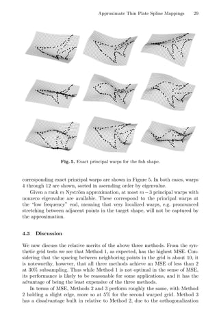
Fig. 4. Approximate principal warps for the fish shape. From left to right and top
to bottom, the surfaces are ordered by eigenvalue in increasing order. The first three
principal warps, which represent the affine component of the transformation and have
eigenvalue zero, are not shown.
where
ˆΛ
∆
= Σ−1
+ Σ−1
V T
PS−1
PT
V Σ−1
= WDWT
to obtain orthogonal eigenvectors we proceed as in section 3.3 to get
ˆΛ = ˆW ˆΣ ˆWT
where ˆW
∆
= WD1/2
Q ˆΣ1/2
and Q ˆΣQT
is the diagonalization of D1/2
WT
WD1/2
.
Thus we can write
ˆL−1
p = V ˆW ˆΣ ˆWT
V T
An illustration of approximate principal warps for the fish shape is shown
in Figure 4, wherein we have used m = 15 samples. As in [3], the principal
warps are visualized as continuous surfaces, where the surface is obtained by
applying a warp to the coordinates in the plane using a given eigenvector of ˆL−1
p
as the nonlinear spline coefficients; the affine coordinates are set to zero. The

9. Approximate Thin Plate Spline Mappings 29
Fig. 5. Exact principal warps for the fish shape.
corresponding exact principal warps are shown in Figure 5. In both cases, warps
4 through 12 are shown, sorted in ascending order by eigenvalue.
Given a rank m Nystr¨om approximation, at most m−3 principal warps with
nonzero eigenvalue are available. These correspond to the principal warps at
the “low frequency” end, meaning that very localized warps, e.g. pronounced
stretching between adjacent points in the target shape, will not be captured by
the approximation.
4.3 Discussion
We now discuss the relative merits of the above three methods. From the syn-
thetic grid tests we see that Method 1, as expected, has the highest MSE. Con-
sidering that the spacing between neighboring points in the grid is about 10, it
is noteworthy, however, that all three methods achieve an MSE of less than 2
at 30% subsampling. Thus while Method 1 is not optimal in the sense of MSE,
its performance is likely to be reasonable for some applications, and it has the
advantage of being the least expensive of the three methods.
In terms of MSE, Methods 2 and 3 perform roughly the same, with Method
2 holding a slight edge, more so at 5% for the second warped grid. Method 3
has a disadvantage built in relative to Method 2, due to the orthogonalization

10. 30 G. Donato and S. Belongie
(a) (b)
Fig. 6. Comparison of Method 2 (a) and 3 (b) for poorly chosen sample locations. (The
performance of Method 1 was terrible and is not shown.) Both methods perform well
considering the location of the samples. Note that the error is slightly lower for Method
3, particularly at points far away from the samples.
step; this leads to an additional loss in significant figures and a slight increase
in MSE. In this regard Method 2 is the preferred choice.
While Method 3 is comparatively expensive and has slightly higher MSE
than Method 2, it has the benefit of providing approximate eigenvectors of the
bending energy matrix. Thus with Method 3 one has the option of studying
shape transformations using principal warp analysis.
As a final note, we have observed that when the samples are chosen badly,
e.g. crowded into a small area, Method 3 performs better than Method 2. This is
illustrated in Figure 6, where all of the samples have been chosen at the back of
the tail fin. Larger displacements between corresponding points are evident near
the front of the fish for Method 2. We have also observed that the bending energy
estimate of Method 2 ( ˜wT
A ˜w) exhibits higher variance than that of Method 3;
e.g. at a 20% sampling rate on the fish shapes warped using If = 0.3 over 100
trials, Method 2 estimates If to be 0.29 with σ = 0.13 whereas Method 3 gives
0.25 and σ = 0.06. We conjecture that this advantage arises from the presence
of the approximate basis functions in the Nystr¨om approximation, though a
rigorous explanation is not known to us.
5 Conclusion
We have discussed three approximate methods for recovering TPS mappings
between 2D pointsets that greatly reduce the computational burden. An exper-
imental comparison of the approximation error suggests that the two methods
that use only a subset of the available correspondences but take into account the
full set of target values perform very well. Finally, we observed that the method
based on the Nystr¨om approximation allows for principal warp analysis and per-

11. Approximate Thin Plate Spline Mappings 31
forms better than the basis-subset method when the subset of correspondences
is chosen poorly.
Acknowledgments. The authors wish to thanks Charless Fowlkes, Jitendra
Malik, Andrew Ng, Lorenzo Torresani, Yair Weiss, and Alice Zheng for helpful
discussions. We would also like to thank Haili Chui and Anand Rangarajan for
useful insights and for providing the fish datasets.
Appendix: Generating Random TPS Transformations
To produce a random TPS transformation with bending energy ν, first choose a
set of p reference points (e.g. on a grid) and form L−1
p . Now generate a random
vector u, set its last three components to zero, and normalize it. Compute the
diagonalization L−1
p = UΛUT
, with the eigenvalues sorted in descending order.
Finally, compute w =
√
νUΛ1/2
u. Since If is unaffected by the affine terms,
their values are arbitrary; we set translation to (0, 0) and scaling to (1, 0) and
(0, 1).
References
1. C. T. H. Baker. The numerical treatment of integral equations. Oxford: Clarendon
Press, 1977.
2. S. Belongie, J. Malik, and J. Puzicha. Matching shapes. In Proc. 8th Int’l. Conf.
Computer Vision, volume 1, pages 454–461, July 2001.
3. F. L. Bookstein. Principal warps: thin-plate splines and decomposition of defor-
mations. IEEE Trans. Pattern Analysis and Machine Intelligence, 11(6):567–585,
June 1989.
4. H. Chui and A. Rangarajan. A new algorithm for non-rigid point matching. In
Proc. IEEE Conf. Comput. Vision and Pattern Recognition, pages 44–51, June
2000.
5. M.H. Davis, A. Khotanzad, D. Flamig, and S. Harms. A physics-based coordinate
transformation for 3-d image matching. IEEE Trans. Medical Imaging, 16(3):317–
328, June 1997.
6. F. Girosi, M. Jones, and T. Poggio. Regularization theory and neural networks
architectures. Neural Computation, 7(2):219–269, 1995.
7. M. J. D. Powell. A thin plate spline method for mapping curves into curves in two
dimensions. In Computational Techniques and Applications (CTAC95), Melbourne,
Australia, 1995.
8. A.J. Smola and B. Sch¨olkopf. Sparse greedy matrix approximation for machine
learning. In ICML, 2000.
9. G. Wahba. Spline Models for Observational Data. SIAM, 1990.
10. Y. Weiss. Smoothness in layers: Motion segmentation using nonparametric mixture
estimation. In Proc. IEEE Conf. Comput. Vision and Pattern Recognition, pages
520–526, 1997.
11. C. Williams and M. Seeger. Using the Nystr¨om method to speed up kernel ma-
chines. In T. K. Leen, T. G. Dietterich, and V. Tresp, editors, Advances in Neural
Information Processing Systems 13: Proceedings of the 2000 Conference, pages
682–688, 2001.