Downloaded 22 times
![number of possible results are equality likely. This is the classical or ;”a priori” approach. The
phrase “ a priori” comes from Latin words meaning coming from what was known before. This
approach is often simple to visualize, so giving a better understanding of probability. In some cases it
can be applied directly in engineering.
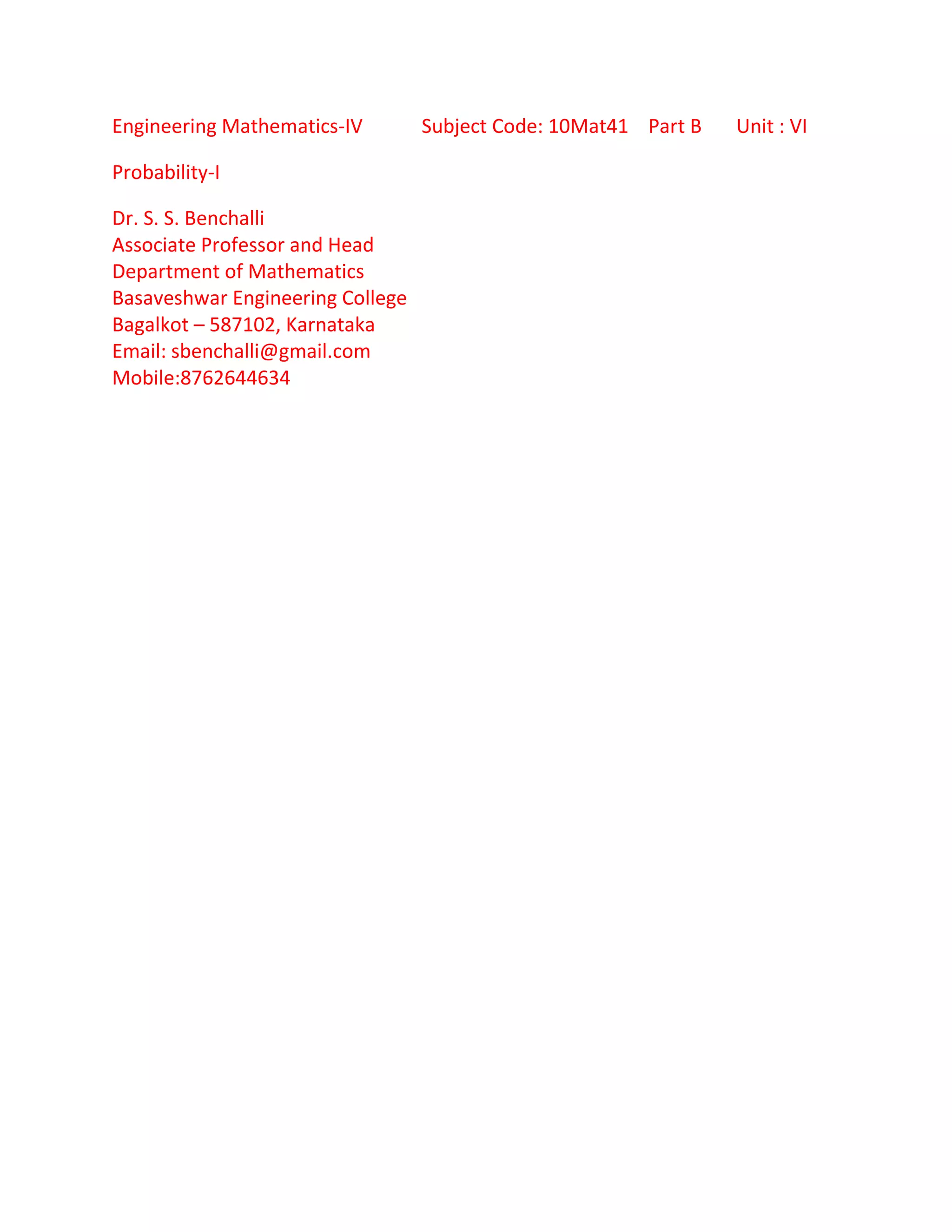
Example: Two fair coins are tossed. What is the probability of getting one heads and one tails?
Answer: For a fair or unbiased coin, for each toss of each coin P[heads] =P[tails] = ½
This assumes that all other possibilities are excluded: if a coin is lost that toss will be eliminated.
The possibility that a coin will stand on edge after tossing can be neglected.
There are two possible results of tossing the first coin. These are heads (H) and tails (T), and
they are equally likely. Whether the result of tossing the first coin is heads or tails, there are
two possible results of tossing the second coin. Again, these are heads (H) and tails (T), and they
are equally likely. The possible outcomes of tossing the two coins are HH, HT, TH and TT. Since
the results H and T for the first coin are equally likely, and the results H and T for the second
coin are equally likely, the four outcomes of tossing the two coin must be equally likely. These
relationships are conveniently summarized in the following tree diagram. In which each branch
point (or node) represents a point of decision where two or more results are possible.
Outcome
H HH
H
T TT
H TH
T
T TT
Figure: Simple Tree Diagram
Since there are four equally likely outcomes, the probability of each is 1/4. Both HT and TH
correspond to getting one heads and one tails, so two of the four equally likely outcomes give
this result. Then the probability of getting one heads and one tails must be 2/4=1/2 or 0.5.
P[H]=1/2
P[T]=1/2
P[H]=1/2
P[T]=1/2
P[H]=1/2
P[T]=1/2](https://image.slidesharecdn.com/uuni6ssb-140619043834-phpapp01/75/U-uni-6-ssb-4-2048.jpg)
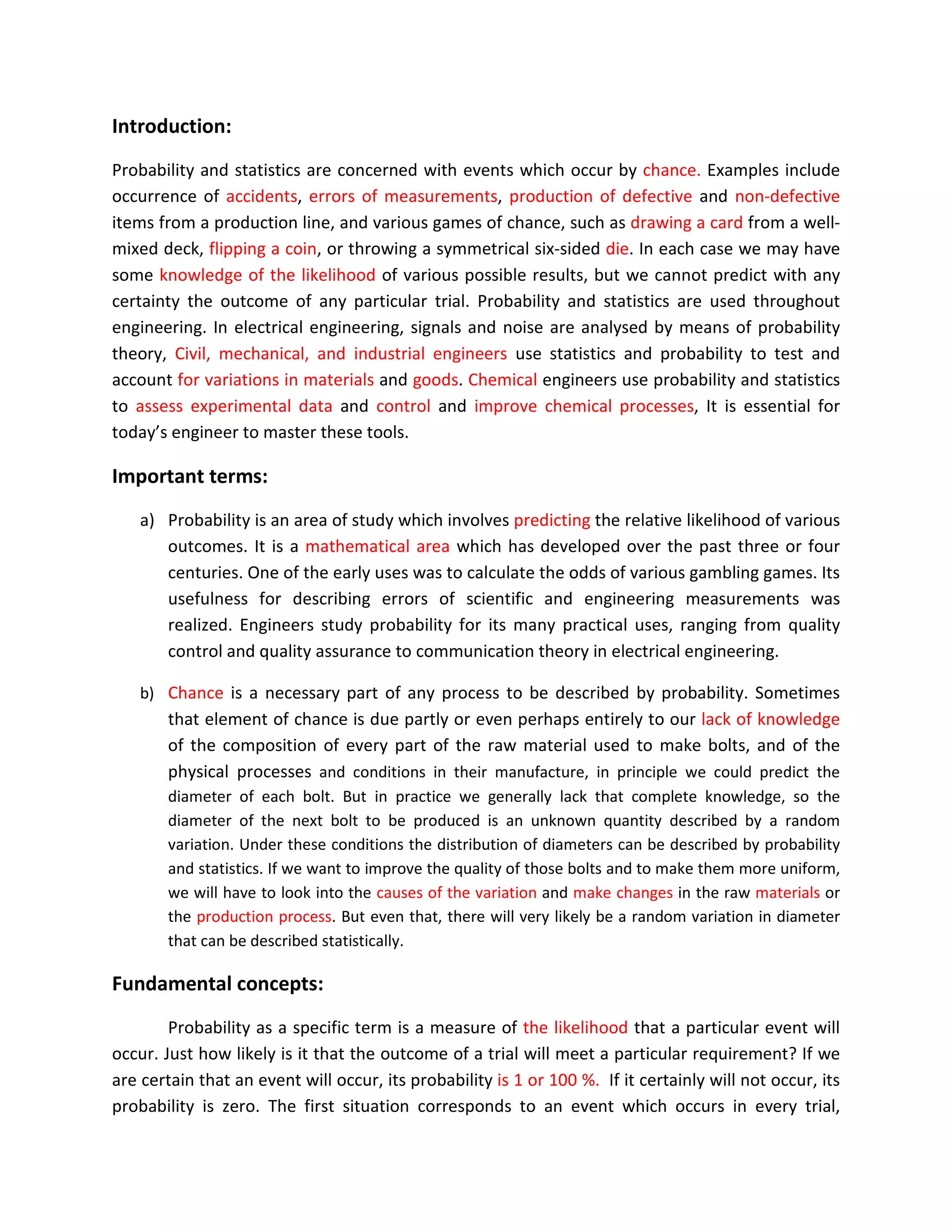
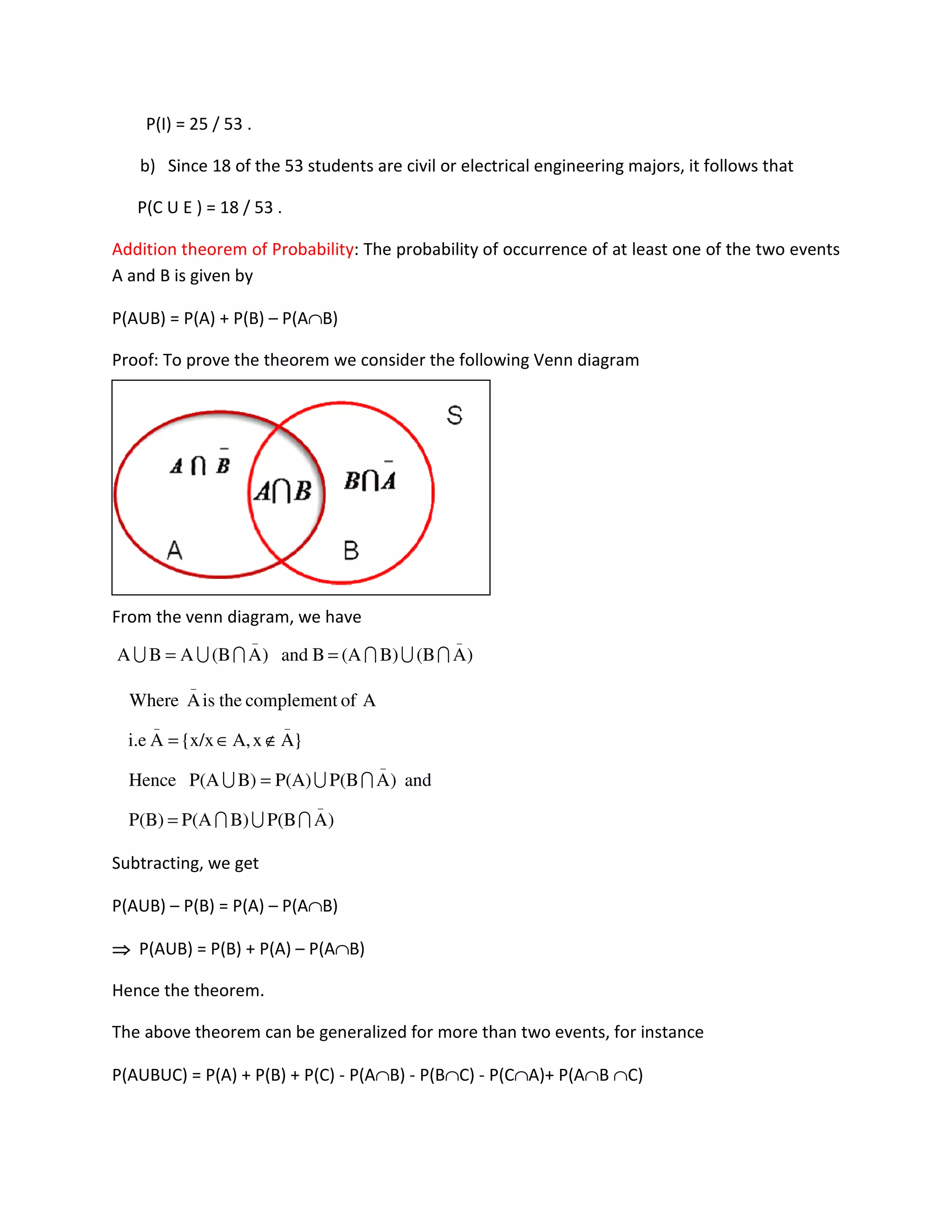
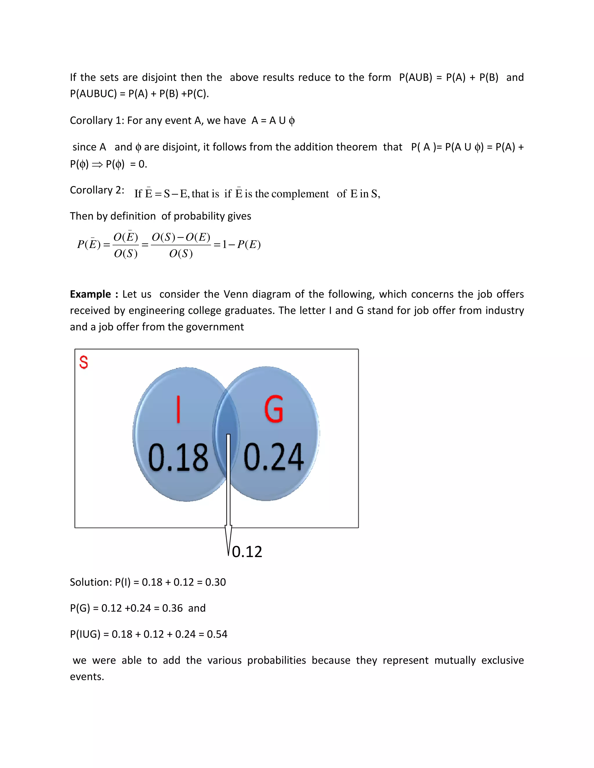
![P (I) = 25 / 53.
b) Since 18 of the 53 students are civil or electrical engineering majors, it follows that
P(C U E) = 18 / 53.
Basic Rules of Combining Probabilities
The basic rules of laws of combining probabilities must be consistent with the
fundamental concepts.
Addition Rule: This can be divided onto two parts, depending upon whether there is overlap
between the events being combined.
a) If the events are mutually exclusive, there is no overlap: if one event occurs, other
events cannot occur. In that case the probability of occurrence of one or another of more than
one event is the sum of the probabilities of the separate events. For example, if I throw a fair
six-sided die the probability of any one face coming up is the same as the probability of any
other face, or one-sixth. There is no overlap among these six possibilities. Then P [6] =1/6, P [4]
=1/6. So P [6 or 4] is 1/6 + 1/6 = 1/3. This, then, is the probability of obtaining a six or a four on
throwing one dir. Notice that it is consistent with the classical approach to probability; of six
equally likely results, two give the result which was specified. The addition rule corresponds to
a logical or and gives a sum of separate probabilities.
Often we can divide all possible outcomes into two groups without overlap. If one group of
outcomes is event A, the other group is the complement of A and is written
_
A or A’. Since A
and
_
A together include all possible results, the sum of P[A] and P[
_
A ] must be 1. If P[
_
A ] is
more easily calculated than P[A], the best approach to calculating P[A] may be by first
calculating P[
_
A ].
Example: A sample of four electronic components is taken from the output of a production line.
The probabilities of the various outcomes are calculated to be; P [0 defectives]=0.6561. P [1
defective] = 0.2916, P [2 defective] = 0.0486. P [3 defective] = 0.0036. P [4 defective] = 0.0001.
What is the probability of at least one defective?
Answer: If would be perfectly correct to calculate as follows:
P[ at least one defective ] = P[ 1 defective ]+ P[ 2 defective ]+ P[ 3 defective ]+ P[ 4 defective ]
= 0.2916 + 0.0486 + 0.0036 + 0.0001 = 0.3439.](https://image.slidesharecdn.com/uuni6ssb-140619043834-phpapp01/75/U-uni-6-ssb-6-2048.jpg)
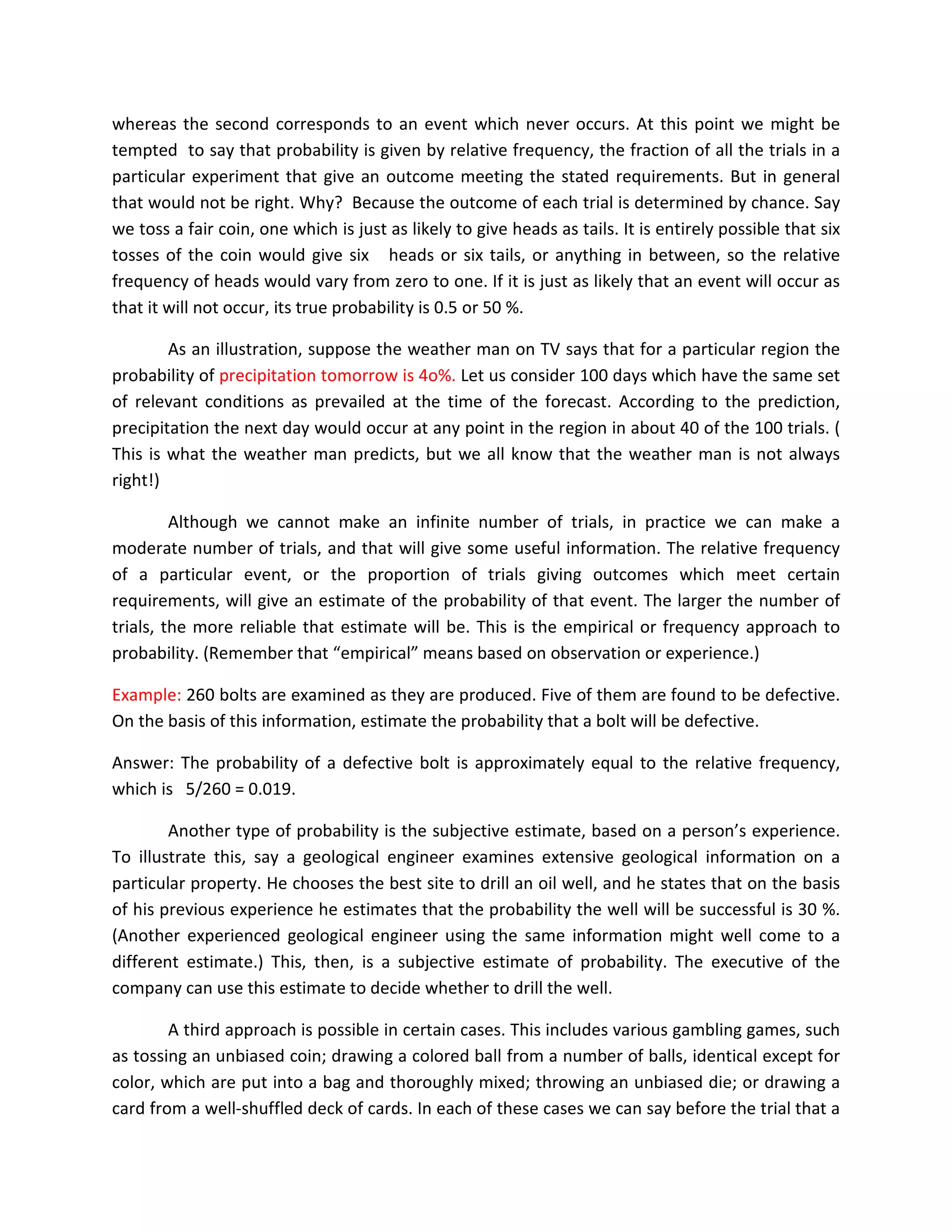
![But is is easier to calculate instead:
P [ at least one defective ] = 1- P [ 0 defective ]
= 1 – 0.6561
= 0.3439 or 0.344.
b) If the events are not mutually exclusive, there can be overlap between them. This can
be visualized using a VENN diagram. The probability of overlap must be subtracted from
the sum of probabilities of the separate events ( i.e, we must not count the same area
on the Vann Diagram twice).
Figure: Venn diagram
The circle marked A represents the probability (or frequency) of event A, the circle marked B
represents the probability (or frequency) of event B, and the whole rectangle represents all
possibilities, so a probability of one or the total frequency. The set consisting of all possible
outcomes of a particular experiment is called the sample space of that experiment. Thus, the
rectangle on the Venn diagram corresponds to the sample space. An event, such as A or B, is
any subset of a sample space.
Set notation is useful:
P[AUB]=P[Occurrence of A or B or Both], the union of the two events A and B
P[A∩ B] = P[Occurrence of both A and B ], the intersection of events A and B. Then in above
figure, the intersection A∩ B represents the overlap between events A and B.
The following Venn diagram representing intersection, union, and completement. The cross-
hatched area of Figure (a) represents event A. The cross-hatched area of Figure (b) shows the
intersection of events A and B. The union of events A and B is shown on part (c) of the diagram.
The cross-hatched area of part ( d ) represents the complement of event A’.
A B
A∩ B](https://image.slidesharecdn.com/uuni6ssb-140619043834-phpapp01/75/U-uni-6-ssb-7-2048.jpg)
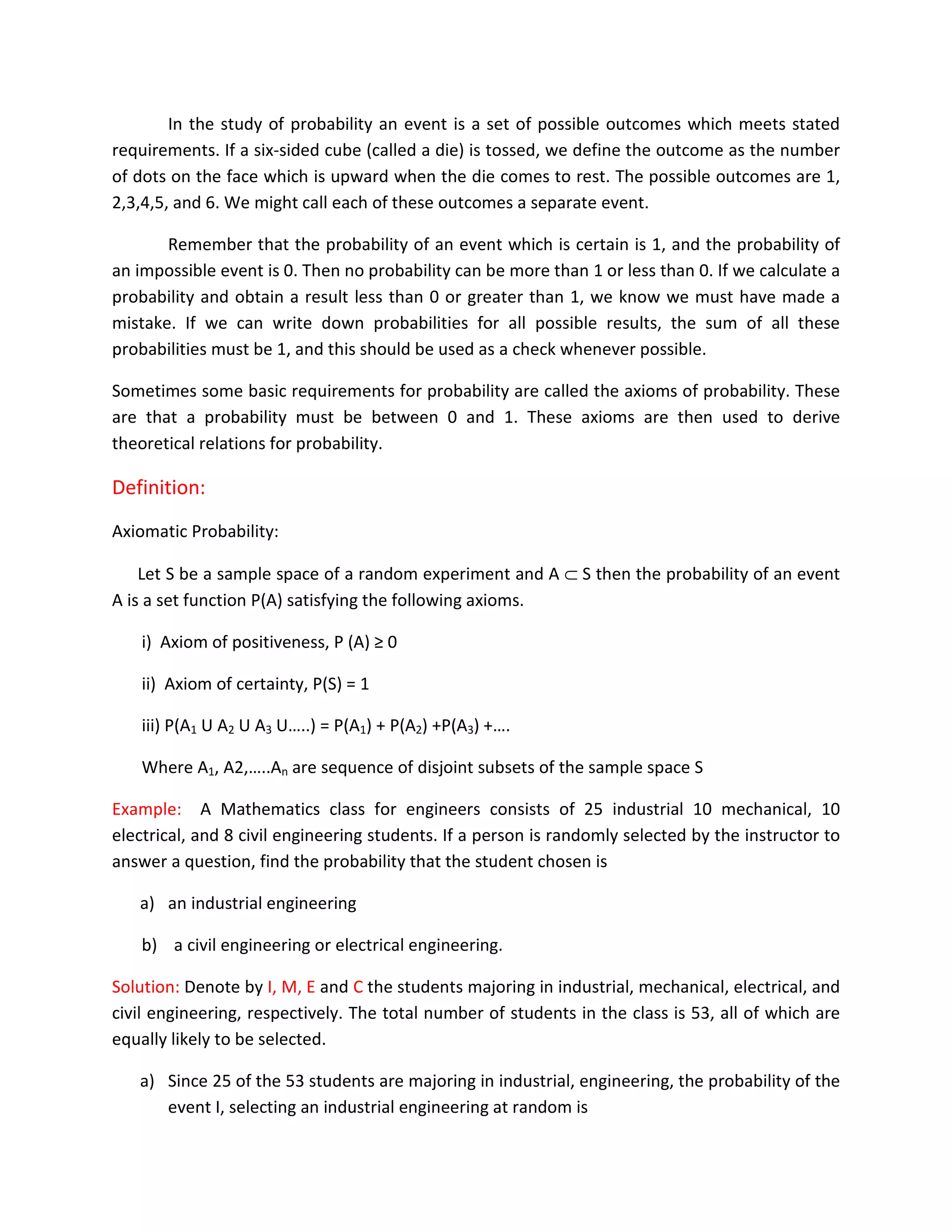
![(a) Event A (b) Intersection
( C) Union (d) Complement
Figure: Relations on Venn Diagrams
If the events being considered are not mutually exclusive, and so there may be overlap
between them, the Addition Rule becomes
P(AUB) = P[A] +P[B} –P[A∩B] In words, the probability of A or B or both is the sum of the
probabilities of A and of B, less the probability of the overlap between A and B. The overlap is
the intersection between A and B.
Example: A Mathematics class for engineers consists of 25 industrial 10 mechanical, 10
electrical, and 8 civil engineering students. If a person is randomly selected by the instructor to
answer a question, find the probability that the student chosen is
a) an industrial engineering
b) a civil engineering or electrical engineering.
Solution: Denote by I,M,E and C the students majoring in industrial, mechanical, electrical, and
civil engineering, respectively. The total number of students in the class is 53, all of which are
equally likely to be selected.
a) Since 25 of the 53 students are majoring in industrial, engineering, the probability of the
event I, selecting an industrial engineering at random is
A A B
A B A’
A](https://image.slidesharecdn.com/uuni6ssb-140619043834-phpapp01/75/U-uni-6-ssb-8-2048.jpg)
![Now
P[(B1 ∩ B2 ) or (W1 ∩ B2)] = P(B1 ∩ B2 ) + P (W1 ∩ B2)
= P(B1) P(B2/B1) + P(W1) P(B2/W1)
= (3/7) (6/9) + (4/7) (5/9)
= 38 / 63.
Theorem: Two events A and B are independent if and only if
P(A ∩ B) =P(A) P(B)
Therefore, to obtain the probability that two independent events will both occur, we simply
find the product of their individual probabilities.
Example: A small town has one fire engine and one ambulance available for emergencies.The
probability that the fire engine is available when needed is 0.98, and the probability that the
ambulance is available when called is 0.92. In the event of an injury resulting from a burning
building, find the probability that both the ambulance and the fire engine will be available.
Bag1
4W 3B
B1 3/7
W1
4/7
B2 6/9 P(B1∩B2)=(3/7)(6/9)
P(B ∩B )=(3/7)(6/9)
W2 3/9 P(B1∩W2)=(3/7)(3/9)
B2 5/9 P(W1∩B2)=(4/7)(5/9)
W2 4/9 P(W1∩W2)=(4/7)(4/9)](https://image.slidesharecdn.com/uuni6ssb-140619043834-phpapp01/75/U-uni-6-ssb-16-2048.jpg)
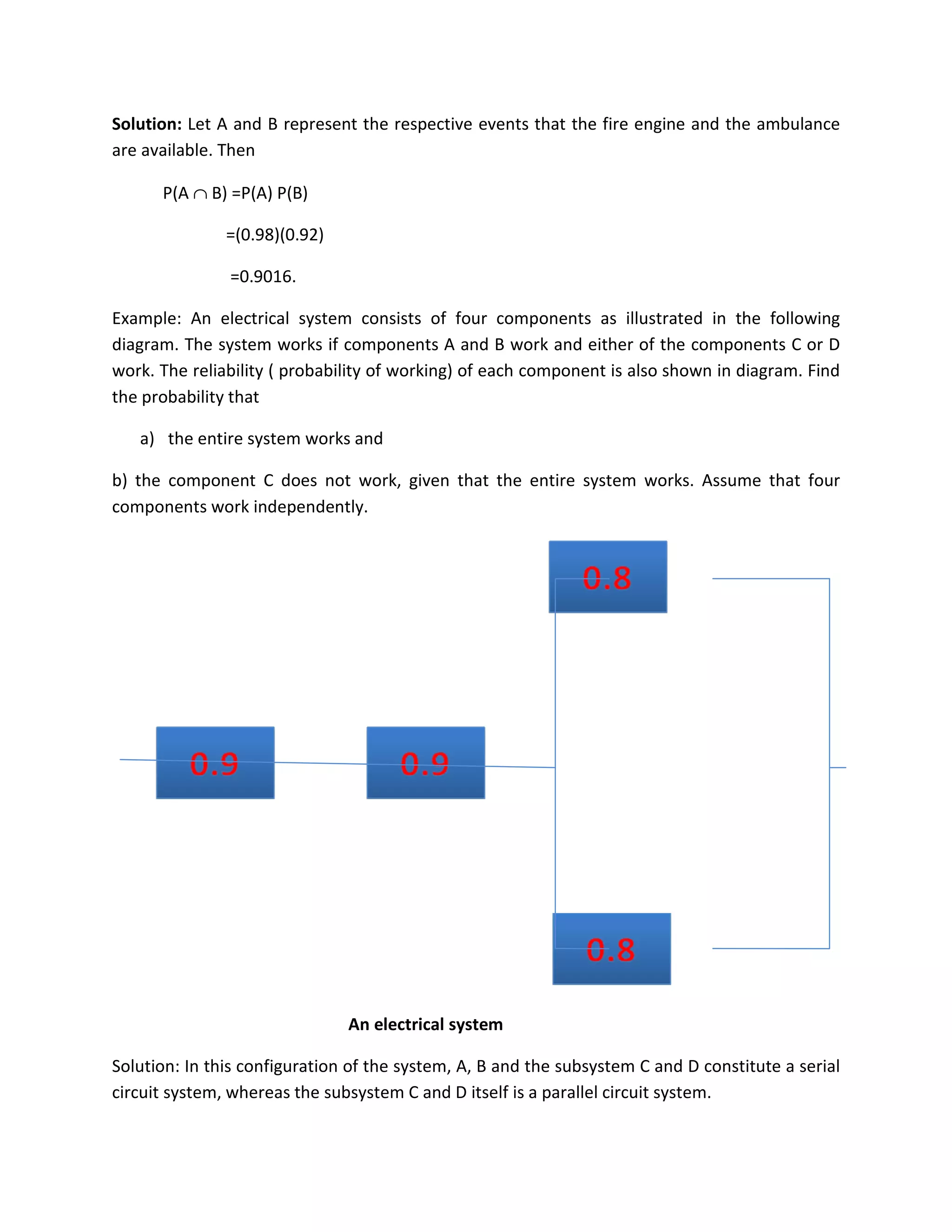
![a) Clearly the probability that the entire system works can be calculated as the following:
P(A∩B∩(CUD)) = P(A) P(B) P(CUD)
= P(A) P(B) [1 – P(C’ ∩ D ‘ )]
= P(A)P(B) [1 – P(C’ )P(D’)]
= (0.9)(0.9)[1-(1-0.8)(1-0.8)]
= 0.7776.
The equalities above hold because of the independence among the four components.
b) To calculate the conditional probability in this case, notice that
Bayes’ Theorem: The general multiplication rules are useful in solving many problems in which
the ultimate outcome of an experiment depends on the outcomes of various intermediate
stages.
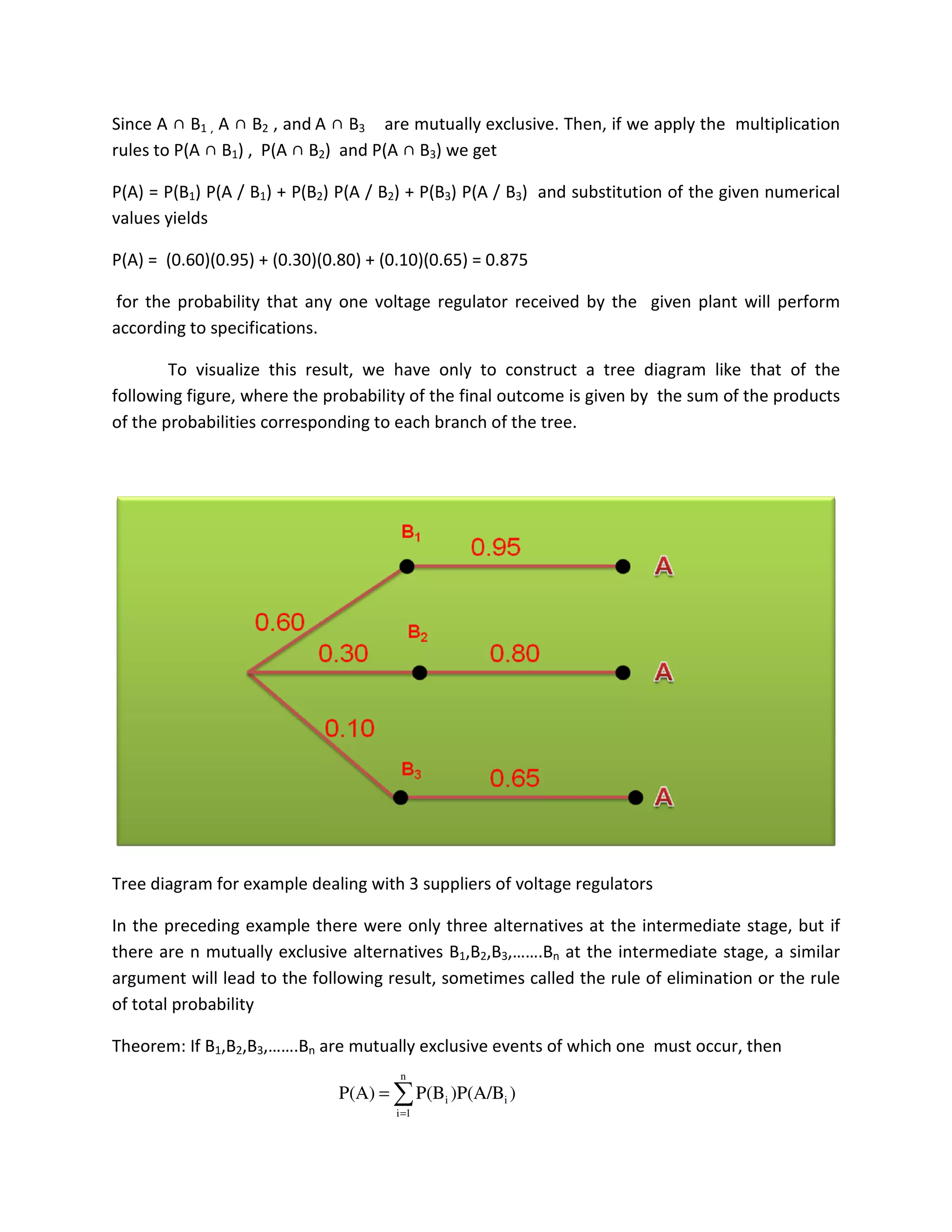
Suppose, for instance, that an assembly plant receives its voltage regulators from three
different suppliers, 60 % from supplier B1, 30 % from supplier B2, and 10 % from supplier B3.
In other words, the probabilities that any one voltage regulator received by the plant
comes from these three suppliers are 0.60, 0.30, and 0.10.
If 95% of the voltage regulators from B1, 80 % of those from B2, and 65 % of those from B3
perform according to specifications, what we would like to know is the probability that any one
voltage regulator received by the plant will perform according to specifications
If A denotes the event that a voltage regulator received by the plant performs according to
specifications, and B1,B2, and B3 are the events that it comes from the respective suppliers, we
can write A = A∩[B1∪B2 ∪ B3 ]
= (A ∩ B1) ∪ (A ∩ B2)∪ (A ∩ B3) and
P(A) = P(A ∩ B1) + P(A ∩ B2) + P(A ∩ B3)
.1667.0
7776.0
)8.0)(8.01)(9.0)(9.0(
works)systemP(the
D)'CBP(A
works)systemP(the
not work)doesCbutworkssystemP(the
P
=
−
=
=
=
III](https://image.slidesharecdn.com/uuni6ssb-140619043834-phpapp01/75/U-uni-6-ssb-18-2048.jpg)


This document provides an introduction to probability and important concepts in probability theory. It defines probability as a measure of the likelihood of an event occurring based on chance. Probability can be estimated empirically by calculating the relative frequency of outcomes in a series of trials, or estimated subjectively based on experience. Classical probability uses an a priori approach to assign probabilities to outcomes that are considered equally likely, such as outcomes of rolling dice or drawing cards. The document provides examples and definitions of key probability terms and concepts such as sample space, events, axioms of probability, and approaches to calculating probability.


