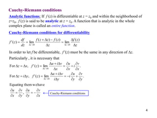
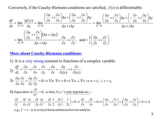
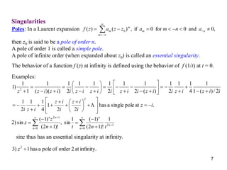
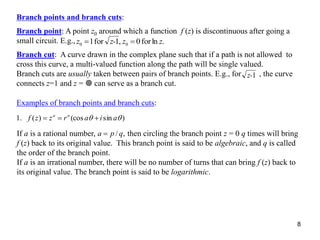
This document discusses functions of complex variables. It defines key concepts such as complex numbers, the Cauchy-Riemann conditions for differentiability, and analytic functions. The Cauchy-Riemann conditions require the partial derivatives of the real and imaginary parts of a complex function to satisfy certain relationships. Functions that satisfy the Cauchy-Riemann conditions everywhere are said to be analytic. The document also discusses singularities such as poles and essential singularities.

1. 1
Functions of a Complex Variable
Sumita Gulati
Assistant Professor
S. A. Jain College, Ambala City

2. Complex number:
Complex algebra:
Complex conjugation:
2
.)1real,areand(both  iyxiyxz
Cauchy-Riemann conditions
Complex algebra
Functions of a Complex Variable
       
           2112212121221121
2121221121 vectors.)2dto(Anologous
zzicycxiyxcczyxyxiyyxxiyxiyxzz
yyixxiyxiyxzz


iyxiyxz  **
)(
22*
))(( yxiyxiyxzz 
Modulus (magnitude): 2121
22*
zzzzyxrzzz 
Polar representation: 
 i
reiriyxz  )sin(cos
Argument (phase):
)arg()arg()arg(
)quadrants.3rdor2ndin theisif(arctan)arg(
2121 zzzz
z
x
y
z







 

3. 3
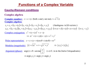
Functions of a complex variable:
All elementary functions of real variables may be extended into the complex plane.






0
2
0
2
!!2!1
1
!!2!1
1:Example
n
n
z
n
n
x
n
zzz
e
n
xxx
e 
A complex function can be resolved into its real part and imaginary part:
2222
2222
11
2)()(:Examples
),(),()(
yx
y
i
yx
x
iyxz
xyiyxiyxz
yxivyxuzf









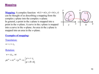
Multi-valued functions and branch cuts:
ivunirrerez nii
 
)2(ln]ln[)ln(ln:1Example )2(

To remove the ambiguity, we can limit all phases to (-,).
 = - is the branch cut.
lnz with n = 0 is the principle value.
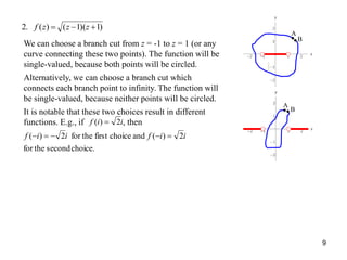
  2/)2(2121)2(2121
)(:2Example  ninii
errerez 

We can let z move on 2 Riemann sheets so that is single valued everywhere.21
)()( i
rezf 

4. 4
Analytic functions: If f (z) is differentiable at z = z0 and within the neighborhood of
z=z0, f (z) is said to be analytic at z = z0. A function that is analytic in the whole
complex plane is called an entire function.
Cauchy-Riemann conditions for differentiability
Cauchy-Riemann conditions
z
zf
z
zfzzf
dz
df
zf
zz 






)(
lim
)()(
lim)('
00
In order to let f be differentiable, f '(z) must be the same in any direction of z.
Particularly , it is necessary that
x
v
y
u
y
v
x
u
y
v
y
u
i
yi
viu
zfyiz
x
v
i
x
u
x
viu
zfxz
y
x






























,
havewethemEquating
.lim)(',For
.lim)(',For
0
0
Cauchy-Riemann conditions
x
v
y
u
y
v
x
u










,

5. 5
Conversely, if the Cauchy-Riemann conditions are satisfied, f (z) is differentiable:
 
.
1
and,lim
limlim
)(
lim
0
000




















































































y
v
i
y
u
ix
v
i
x
u
yix
yix
x
v
i
x
u
yix
y
x
u
i
x
v
x
x
v
i
x
u
yix
y
y
v
i
y
u
x
x
v
i
x
u
z
zf
dz
df
z
zzz
More about Cauchy-Riemann conditions:
1) It is a very strong restraint to functions of a complex variable.
2)
3)
4)
2100 cvcuvuvu
y
v
y
u
x
v
x
u










.
)()( iy
v
i
iy
u
y
u
i
y
v
x
v
i
x
u
dz
df


















analytic.notbutcontinuouseverywhereis,e.g.
000
2
1
2
1
:ondependsonly)(thatso,0toEquivalent
***
*
iyxf
y
v
i
y
u
i
x
v
i
x
u
y
f
i
x
f
iy
f
x
f
z
y
y
f
z
x
x
f
z
f
zz,zf
z
f *



























































6. 6
Cauchy-Riemann conditions:
Our Cauchy-Riemann conditions were derived by requiring f '(z) be the same when z
changes along x or y directions. How about other directions?
Here I do a general search for the conditions of differentiability.
 
 
 
























































































































































x
v
y
u
zf
y
v
x
u
ip
x
u
y
v
i
x
v
y
u
ip
p
y
v
x
v
p
y
u
x
u
iip
y
v
i
y
u
ip
p
y
v
x
v
ip
y
u
x
u
dp
d
dp
zdf
pzf
zp
dx
dy
dx
dy
i
dx
dy
y
v
x
v
i
dx
dy
y
u
x
u
idydx
dy
y
v
dx
x
v
idy
y
u
dx
x
u
idydx
idvdu
dz
df
zf
.conditionsRiemann-Cauchysameget thewe
,directionsallatsamethebe)('requireweifis,That
1
1
1
1
0
)('
.ondependnotdoes)('
hunder whicconditionthefindwant toWe.ofchangetheofdirectionthe,letNow
1
)('
2
2

7. 7
Singularities
Poles: In a Laurent expansion
then z0 is said to be a pole of order n.
A pole of order 1 is called a simple pole.
A pole of infinite order (when expanded about z0) is called an essential singularity.
The behavior of a function f (z) at infinity is defined using the behavior of f (1/t) at t = 0.
Examples:
,0and0for0if,)()( 0  


 nm
m
m
m anmazzazf
12
00
12
1
)!12(
)1(1
sin,
)!12(
)1(
sin)2 





 




 n
n
n
n
nn
tntn
z
z
.atpolesingleahas
22
1
4
11
2
1
2/)(1
1
4
11
2
1
)(2
11
2
111
2
1
))((
1
1
1
)1
2
2
iz
i
iz
i
iz
izi
iiziziiziiziiziziizizz














 































sinz thus has an essential singularity at infinity.
infinity.at2orderofpoleahas1)3 2
z

8. 8
Branch points and branch cuts:
Branch point: A point z0 around which a function f (z) is discontinuous after going a
small circuit. E.g.,
Branch cut: A curve drawn in the complex plane such that if a path is not allowed to
cross this curve, a multi-valued function along the path will be single valued.
Branch cuts are usually taken between pairs of branch points. E.g., for , the curve
connects z=1 and z =  can serve as a branch cut.
.lnfor0,1for1 00 zzz-z 
1z-
Examples of branch points and branch cuts:
)sin(cos)(.1  aiarzzf aa

If a is a rational number, then circling the branch point z = 0 q times will bring
f (z) back to its original value. This branch point is said to be algebraic, and q is called
the order of the branch point.
If a is an irrational number, there will be no number of turns that can bring f (z) back to
its original value. The branch point is said to be logarithmic.
,/ qpa 

9. 9
)1)(1()(.2  zzzf
We can choose a branch cut from z = -1 to z = 1 (or any
curve connecting these two points). The function will be
single-valued, because both points will be circled.
Alternatively, we can choose a branch cut which
connects each branch point to infinity. The function will
be single-valued, because neither points will be circled.
It is notable that these two choices result in different
functions. E.g., if , theniif 2)( 
choice.secondfor the
2)(andchoicefirstfor the2)( iifiif 
A
B
A
B

10. 10
Mapping
Mapping: A complex function
can be thought of as describing a mapping from the
complex z-plane into the complex w-plane.
In general, a point in the z-plane is mapped into a
point in the w-plane. A curve in the z-plane is mapped
into a curve in the w-plane. An area in the z-plane is
mapped into an area in the w-plane.
),(),()( yxivyxuzw 
z0
z1
z
y
x
w0
w1
w
v
u
Examples of mapping:
Translation:
0zzw 
Rotation:







0
0
0
0
0
or,


 
rr
erree
zzw
iii

11. 11
Inversion:










 

r
re
e
z
w
i
i
1
1
or,
1
In Cartesian coordinates:
.,
11
22
22
22
22
























vu
v
y
vu
u
x
yx
y
v
yx
x
u
iyx
ivu
z
w
A straight line is mapped into a circle:
.0)( 22
2222






vauvub
b
vu
au
vu
v
baxy

12. 12
Conformal mapping
Conformal mapping: The function w(z) is said to be conformal at z0 if it preserves the
angle between any two curves through z0.
If w(z) is analytic and w'(z0)0, then w(z) is conformal at z0.
Proof: Since w(z) is analytic and w'(z0)0, we can expand w(z) around z = z0 in a
Taylor series:
.)(
).)(('or),('lim
))((''
2
1
))((')(
121200
0000
0
0
0
2
00000
0







zzAeww
zzzwwwzw
zz
ww
zzzwzzzwzww
i
zz

1) At any point where w(z) is conformal, the mapping consists of a rotation and a
dilation.
2) The local amount of rotation and dilation varies from point to point. Therefore a
straight line is usually mapped into a curve.
3) A curvilinear orthogonal coordinate system is mapped to another curvilinear
orthogonal coordinate system .

13. 13
What happens if w'(z0) = 0?
Suppose w (n)(z0) is the first non-vanishing derivative at z0.










 
n
n
Br
reBe
n
ezz
n
zw
ww
n
niiin
n
!)(
!
1
)(
!
)(
0
0
)(
0
This means that at z = z0 the angle between any two curves is magnified by a factor n
and then rotated by .

14. 14
Thank You