SlideShare a Scribd company logo
Hong Li
Deviation of annual temperature in 2014 relative to the 1981-2010 average
Source: Euro4m
Outline
2
 Global Climate Change
 Methods
 Climate Change in Scandinavia
• Temperature
• Precipitation (Extreme & Snow)
 Hydrological Consequence
• Runoff
• Glaciers
Climate
3
Climate describes the average weather over a certain time-span
(usually 30-year period) in a certain location.
Climate Change
4
Statistically significant variations of the mean or variability, typically
persisting for decades or longer.
Temperature, wind, precipitation, humidity, cloud, radiation
Source: IPCC AR3
Global Climate Change
5Data source: NOAA
Global average temperature anomalies 1880 – 2014
1965 – 2014
0.26/decade
0.16/decade
0.12/decade
Changes in annual temperature between
2000 – 2014 and 1961 – 1990
6Source: NASA
Global Climate Change
Zonal mean changes against latitude
Global Climate Change
7
Energy Balance of the Earth
Source: Zolushka, 2015
CO2
Global Climate Change
8
Reconstructed temperature anomalies (°C) relative to present from Vostok and EPICA
Source: ClimateData
‘Milankovitch cycle‘, the changes in the way the earth orbits the sun
9
Source: USGCRP, 2009; IPCC AR5
Concentraion of 3 green house gases
Global Climate Change
Global land surface temperature anomalies
relative to 1880 – 1919
Observations
With human emissions
Without human emissions
1 °C
Global Climate Change
10
Less Sea Ice
Source: EPA
January 2014 Norway
August 2014 Sweden
Outline
11
 Global Climate Change
 Methods
 Climate Change in Scandinavia
• Temperature
• Precipitation (Extreme & Snow)
 Hydrological Consequence
• Runoff
• Glaciers
Methods
Signal Trend Detection
• Linear trend
• Mann-Kendall Test + Sen slope
Future Climate and Impacts
• (AO)GCMs
• RCMs
• Bias Correction/Downscaling
• Hydrological Models (HM)
12
AOGCMs: Atmosphere–Ocean General Circulation Models
RCMs: Regional Climate Models
𝑋 = 𝑎 × 𝑌𝑒𝑎𝑟 + 𝑏
Methods
Future Climate and Impacts
• (AO)GCMs
• RCMs
• Bias Correction/Downscaling
• Hydrological Models (HM)
13
Source: Bice, 2015
10-20 layers
20 layers
100 – 600 km
Methods
14Source: ConsulClima
Future Climate and Impacts
• (AO)GCMs
• RCMs
• Bias Correction/Downscaling
• Hydrological Models (HM)
𝑆𝑀𝑒𝑙𝑡 = 𝑆𝑀𝐸𝐿𝑇𝑅 × 𝑻 − 𝑇𝑚𝑒𝑙𝑡
𝐼𝑀𝑒𝑙𝑡 = 𝐼𝑀𝐸𝐿𝑇𝑅 × (𝑻 − 𝑇𝑚𝑒𝑙𝑡)
P 𝐸 = 𝐸𝑃𝑂𝑇 × 𝑻
𝐴𝐸 =
𝑃𝐸
𝑃𝐸 × 𝑆𝑀 𝐹𝐶 𝐹𝐶𝐷
𝑄0 = 𝐾𝑈𝑍 × 𝑈𝑍 𝛼
𝑄1 = 𝐾𝐿𝑍 × 𝐿𝑍
15
Scheme of the HBV model
Methods
Methods
Advantages
• 4-D global scale simulation
• More climate components
• Finer description of processes
• Increasing resolutions
16
Source: IPCC AR4
Methods
Disadvantages
• Simpler than reality: teleconnections
• Too sparse scales for local processes: extreme events
• Limitations in chemistry and interactions
17
Source: Lupo et al., 2013
Good: fluid motions of atmosphere and oceans
Poor: clouds, dust, chemistry, biology
Good: Temperature
Poor: Precipitation
Outline
18
 Global Climate Change
 Methods
 Climate Change in Scandinavia
• Temperature
• Precipitation (Extreme & Snow)
 Hydrological Consequence
• Runoff
• Glaciers
19
Sweden
450,295 km2; 4.7⁰C/643 mm
Norway
323,802 km2; 1.0⁰C /1104 mm
Denmark
43,094 km2; 7.7⁰C/712 mm
Climate Change in Scandinavia
1961 – 1990
AnnT/AnnP
Fast warming
• 0.26 °C/decade Global Land
• 0.37 °C/decade in Norway
• 0.36 °C/decade in Sweden
(a)
(b) (c)
Source: Drange, 2015; SMHI; DMI
Temperature
20
(a) Norway (relative to 1901 – 2000 mean)
(b) Sweden (relative to 1961 – 1990 mean)
(c) Denmark
-/0.36 °C/decade
Temperature
21
Seasonal difference
• More increase in Winter
• Less increase in Summer
Source: Nilsen, 2015
Monthly temperature changes
over the 31-year periods for mainland Norway
Temperaturechange(°C)
Temperature
22
Spatial variation
• More increase in North
• Less increase in South
Temperature trend (°C/decade) in January
Watch Forcing Data ERA-Interim
1979 – 2009
Source: Irene, 2015
Temperature
23
Temperature change (°C) in 2071 – 2100 relative to 1971 – 2000 by 9 GCMs, RCA4, Rcp8.5
Source: SMHI
Annual Winter Summer
More precipitation
• 18/31% per 100 yr in Norway
• 17/34% per 100 yr in Sweden
24
(a)
(b) (c)
Source: Drange, 2015; SMHI, DMI
Precipitation
(a) Norway (relative to 1901 – 2000 mean)
(b) Sweden
(c) Denmark
17/34 % per 100 yr
Precipitation
25
Seasonal difference
• More increase in winter and less in summer
Source: Drange, 2015
Change in precipitation in Norway (relative to 1901 – 2000)
(a) winter (b) summerWinter Summer
Relative increase in annual precipitation
1990 – 2003 to 1961 – 1990
Spatial variation
• More increase in North and West Norway.
Precipitation
26Source: : Thorsteinsson & Björnsson, 2011
Precipitation
27
Annual Winter Summer
Relative change (%) in 2071 – 2100 to 1971 – 2000 by 9 GCMs, RCA4, Rcp8.5
Source: SMHI
Precipitation: Extreme
Yearly Maximum 1 day
28
Mean of yearly maximum precipitation (bars) based on 60 long-
term stations in Sweden. Red curve is smoothed value. Dotted
black curve smoothed value based on 740 stations.
Trend (% per decade) in 1900 – 2004
relative to 1961 – 1990
Source: SMHI; Alfnes & Førland, 2006
Precipitation: Extreme
29
Sub-daily
Relative change in 10-year rainfall amount (1981 – 2010) averaged over Sweden in the projections.
Vertical line represents ± one standard deviation. Grey symbol represents a change that is not statistically
significant.
2011 – 2040 2071 – 2100
Source: Olsson & Foster, 2014
Precipitation: Snow
Less snow days
30Source: Dyrrdal, 2009
Linear trend in No. of snow days for all observations
10 statistically positive (low temperature)
247 statistically negative
Stronger in southeast and southern coast
Stronger after 1990
No./year
Precipitation: Snow
Less snow depth
31Source: Dyrrdal, 2009
No. of snow days Annual mean depth (cm) Max. 1-d increase (cm)
Tunnsjø
Location: (13.6506, 64.6837)
Height: 376 masl
1.9 days/decade
Precipitation: Snow
Less snow in the future
32
Relative change (2071 – 2100 to 1961 – 1990)
By HIRHAM, Hadley, B2
Echam show similar results
altitude
distance from the coast.
Source: Vikhamar-Schuler & Førland, 2006
Precipitation: Snow
Less snow in the future
33
Relative change (2071 – 2100 to 1961 – 1990)
By HBV driven by HIRHAM, Hadley, B2
Echam show similar results
Source: Vikhamar-Schuler & Førland, 2006
Precipitation: Snow
Different between RCM and HM
34
Relative change in SWE
2071 – 2100 to 1961 – 1990
By HBV and HIRHAM
Hadley, B2
HBV
HIRHAM
Below 200 masl
200-1000 masl
Above 1000 masl
Source: Vikhamar-Schuler & Førland, 2006
Outline
35
 Global Climate Change
 Methods
 Climate Change in Scandinavia
• Temperature (increase)
• Precipitation (increase but less Snow)
 Hydrological Consequence
• Runoff
• Glaciers
Water resources, hydropower potential
Limitations of the hydrological models
Flood
Runoff
36
Trends in annual runoff (1961 – 2000)
Source: Wilson et al., 2010
Increase at 95%significance level
Increase at 70%significance level
No trend
Decrease at 70% significance level
Decrease at 95% significance level
Observed annual increase
Runoff
37
Relative increase in annual runoff
1990 – 2003 to 1961 – 1990
Source: Thorsteinsson & Björnsson., 2011
Observed annual increase
Runoff
38
Annual runoff
Source: Thorsteinsson & Björnsson., 2011
Annual precipitation
Runoff
39
More runoff in future
Change in seasonality
Source: JesF, 2007
Daily mean discharge in 2071 – 2100 by four precitions
Source: Beldring et al, 2006
Runoff
40
Annual Winter Spring
Source: Beldring et al, 2006
Runoff
41
Spring Summer Autumn
Runoff
42
Season of annual Max. runoff
25 HBV best parameter sets
8 GCMs, 5RCMs, A2, B2, A1B
Change in flood time
Source: Lawrence & Hisdal, 2011
Runoff
43
Change in flood magnitude
Median change of the change for the
100-year flood in Sweden (%)
2021 – 2050 to 1963 – 1992
Based on 16 regional climate scenarios
Distribution Based Scaling (DBS) approach
1001 river basins.
Source: Thorsteinsson & Björnsson, 2011
Lawrence & Hisdal, 2011 shows similar results in Norway
Runoff
44
Change in flood magnitude
Tora, 263 km2
700 – 2014 masl
North-western
In southern Norway
HBV, HIRHAM5, ECHAM5, A1B
HBV, HIRHAM, HadCM3, A1B
HBV, RCA3, BCM, A1B
100-year flood based on 30-year moving data
Source: Thorsteinsson & Björnsson, 2011
Runoff: Glaciers
45
1960 1970 1980 1990 2000 2010
-3
-2
-1
0
1
2
3
Time (yr)
Massbalance(mw.e.yr
-1
)
Winter Annual Summer
Glacier mass balance of mainland Norway
+1.92
-0.86
-2.78
Source : Engelhardt et al, 2013; Zemp et al, 2010
Cumulative specific mass balance of
Storglaciären.
-0.4 m w.e. yr-1
Runoff: Glaciers
46
coupled mass balance/ice-dynamic or mass-balance/glacier-scaling models
various GCMs, RCMs, A1B
Source: Thorsteinsson & Björnsson, 2011
47
Negative Effects
• Disturb biodiversity
• Affect landscape and tourism
Reasons
• Regrowth
• Climate change
Interactions
Source: Rübberdt; Bryn & Hemsing, 2012; Bryn, 2008
24.6 million m3 per year in 2007 – 2011 in Norway
48
Evaporation and cloud
• Heat flux
• Water vapour
• Increase reflection
Absorb carbon
Reduce albedo
Interactions
Source: DeWit et al, 2014
Summary
 Temperature
• Has increased more than 0.35°C/decade in Norway and Sweden (1965 – 2014)
• Will very likely amplify in future (more than 0.5°C/decade Rcp8.5)
Precipitation
• Has increased more than 30% in Norway and Sweden (1965 – 2014)
• Will likely increase in the future and less snow
Runoff
• Has increased and will continue with more glacier melting
• Large spatial variations and change in seasonality
49

More Related Content

What's hot

Combining Oceanic And Atmospheric Carbon Data to constrain CO2 fluxes in Europ...
Combining Oceanic And Atmospheric Carbon Data to constrain CO2 fluxes in Europ...Combining Oceanic And Atmospheric Carbon Data to constrain CO2 fluxes in Europ...
Combining Oceanic And Atmospheric Carbon Data to constrain CO2 fluxes in Europ...
Integrated Carbon Observation System (ICOS)
 
Bottom-up and top-down methods in national GHG emission reporting
Bottom-up and top-down methods in national GHG emission reportingBottom-up and top-down methods in national GHG emission reporting
Bottom-up and top-down methods in national GHG emission reporting
Integrated Carbon Observation System (ICOS)
 
Ccss j merrill_overview-1
Ccss j merrill_overview-1Ccss j merrill_overview-1
Ccss j merrill_overview-1
riseagrant
 
Some Developments in Climate Science Since IPCC AR4 Prepared for the Climate ...
Some Developments in Climate Science Since IPCC AR4 Prepared for the Climate ...Some Developments in Climate Science Since IPCC AR4 Prepared for the Climate ...
Some Developments in Climate Science Since IPCC AR4 Prepared for the Climate ...
riseagrant
 
Dibas shrestha
Dibas shresthaDibas shrestha
Dibas shresthaClimDev15
 
Althuizen, Inge: Annual ecosystem carbon budgets across an abrupt permafrost ...
Althuizen, Inge: Annual ecosystem carbon budgets across an abrupt permafrost ...Althuizen, Inge: Annual ecosystem carbon budgets across an abrupt permafrost ...
Althuizen, Inge: Annual ecosystem carbon budgets across an abrupt permafrost ...
Integrated Carbon Observation System (ICOS)
 
Macharia, Joseph - Climate Food and Farming CLIFF Network annual workshop Nov...
Macharia, Joseph - Climate Food and Farming CLIFF Network annual workshop Nov...Macharia, Joseph - Climate Food and Farming CLIFF Network annual workshop Nov...
Macharia, Joseph - Climate Food and Farming CLIFF Network annual workshop Nov...
CCAFS | CGIAR Research Program on Climate Change, Agriculture and Food Security
 
IndiceHong
IndiceHongIndiceHong
IndiceHongHong Li
 
Thompson, Rona: Changes in Net Ecosystem Exchange over Europe During the 2018...
Thompson, Rona: Changes in Net Ecosystem Exchange over Europe During the 2018...Thompson, Rona: Changes in Net Ecosystem Exchange over Europe During the 2018...
Thompson, Rona: Changes in Net Ecosystem Exchange over Europe During the 2018...
Integrated Carbon Observation System (ICOS)
 
Impact of Sea Level Rise from Storm Surge USA
Impact of Sea Level Rise from Storm Surge USAImpact of Sea Level Rise from Storm Surge USA
Impact of Sea Level Rise from Storm Surge USA
Dag Lohmann
 
How is the Greenland ice sheet behaving under global warming and what are the...
How is the Greenland ice sheet behaving under global warming and what are the...How is the Greenland ice sheet behaving under global warming and what are the...
How is the Greenland ice sheet behaving under global warming and what are the...
Meg Stewart
 
GLOBAL WARMING CAUSES FLOOD & DROUGHT
GLOBAL WARMING CAUSES FLOOD & DROUGHTGLOBAL WARMING CAUSES FLOOD & DROUGHT
GLOBAL WARMING CAUSES FLOOD & DROUGHT
Sami Asokan
 
Quantification of urban CO2 emissions
Quantification of urban CO2 emissionsQuantification of urban CO2 emissions
Quantification of urban CO2 emissions
Integrated Carbon Observation System (ICOS)
 
Constraining terrestrial carbon fluxes by assimilating the SMOS soil moisture...
Constraining terrestrial carbon fluxes by assimilating the SMOS soil moisture...Constraining terrestrial carbon fluxes by assimilating the SMOS soil moisture...
Constraining terrestrial carbon fluxes by assimilating the SMOS soil moisture...
Integrated Carbon Observation System (ICOS)
 
Organizzazione meteorologica mondiale, il report 2015
Organizzazione meteorologica mondiale, il report 2015Organizzazione meteorologica mondiale, il report 2015
Organizzazione meteorologica mondiale, il report 2015
Agi
 
Keppler, Lydia: Reconstructing sub-surface Dissolved Inorganic Carbon from ob...
Keppler, Lydia: Reconstructing sub-surface Dissolved Inorganic Carbon from ob...Keppler, Lydia: Reconstructing sub-surface Dissolved Inorganic Carbon from ob...
Keppler, Lydia: Reconstructing sub-surface Dissolved Inorganic Carbon from ob...
Integrated Carbon Observation System (ICOS)
 
Global warming & Various Aspects
Global warming & Various AspectsGlobal warming & Various Aspects
Global warming & Various Aspects
Abhishek Mahajan
 
Forest net ecosystem CO2 exchange in sloping terrain as derived by eddy covar...
Forest net ecosystem CO2 exchange in sloping terrain as derived by eddy covar...Forest net ecosystem CO2 exchange in sloping terrain as derived by eddy covar...
Forest net ecosystem CO2 exchange in sloping terrain as derived by eddy covar...
Integrated Carbon Observation System (ICOS)
 
Regional changes in land-atmosphere CO2 exchange over recent decades using DGVMs
Regional changes in land-atmosphere CO2 exchange over recent decades using DGVMsRegional changes in land-atmosphere CO2 exchange over recent decades using DGVMs
Regional changes in land-atmosphere CO2 exchange over recent decades using DGVMs
Integrated Carbon Observation System (ICOS)
 
Key Findings of the IPCC WG1 Fifth Assessment Report
Key Findings of the IPCC WG1 Fifth Assessment ReportKey Findings of the IPCC WG1 Fifth Assessment Report
Key Findings of the IPCC WG1 Fifth Assessment Report
Katestone
 

What's hot (20)

Combining Oceanic And Atmospheric Carbon Data to constrain CO2 fluxes in Europ...
Combining Oceanic And Atmospheric Carbon Data to constrain CO2 fluxes in Europ...Combining Oceanic And Atmospheric Carbon Data to constrain CO2 fluxes in Europ...
Combining Oceanic And Atmospheric Carbon Data to constrain CO2 fluxes in Europ...
 
Bottom-up and top-down methods in national GHG emission reporting
Bottom-up and top-down methods in national GHG emission reportingBottom-up and top-down methods in national GHG emission reporting
Bottom-up and top-down methods in national GHG emission reporting
 
Ccss j merrill_overview-1
Ccss j merrill_overview-1Ccss j merrill_overview-1
Ccss j merrill_overview-1
 
Some Developments in Climate Science Since IPCC AR4 Prepared for the Climate ...
Some Developments in Climate Science Since IPCC AR4 Prepared for the Climate ...Some Developments in Climate Science Since IPCC AR4 Prepared for the Climate ...
Some Developments in Climate Science Since IPCC AR4 Prepared for the Climate ...
 
Dibas shrestha
Dibas shresthaDibas shrestha
Dibas shrestha
 
Althuizen, Inge: Annual ecosystem carbon budgets across an abrupt permafrost ...
Althuizen, Inge: Annual ecosystem carbon budgets across an abrupt permafrost ...Althuizen, Inge: Annual ecosystem carbon budgets across an abrupt permafrost ...
Althuizen, Inge: Annual ecosystem carbon budgets across an abrupt permafrost ...
 
Macharia, Joseph - Climate Food and Farming CLIFF Network annual workshop Nov...
Macharia, Joseph - Climate Food and Farming CLIFF Network annual workshop Nov...Macharia, Joseph - Climate Food and Farming CLIFF Network annual workshop Nov...
Macharia, Joseph - Climate Food and Farming CLIFF Network annual workshop Nov...
 
IndiceHong
IndiceHongIndiceHong
IndiceHong
 
Thompson, Rona: Changes in Net Ecosystem Exchange over Europe During the 2018...
Thompson, Rona: Changes in Net Ecosystem Exchange over Europe During the 2018...Thompson, Rona: Changes in Net Ecosystem Exchange over Europe During the 2018...
Thompson, Rona: Changes in Net Ecosystem Exchange over Europe During the 2018...
 
Impact of Sea Level Rise from Storm Surge USA
Impact of Sea Level Rise from Storm Surge USAImpact of Sea Level Rise from Storm Surge USA
Impact of Sea Level Rise from Storm Surge USA
 
How is the Greenland ice sheet behaving under global warming and what are the...
How is the Greenland ice sheet behaving under global warming and what are the...How is the Greenland ice sheet behaving under global warming and what are the...
How is the Greenland ice sheet behaving under global warming and what are the...
 
GLOBAL WARMING CAUSES FLOOD & DROUGHT
GLOBAL WARMING CAUSES FLOOD & DROUGHTGLOBAL WARMING CAUSES FLOOD & DROUGHT
GLOBAL WARMING CAUSES FLOOD & DROUGHT
 
Quantification of urban CO2 emissions
Quantification of urban CO2 emissionsQuantification of urban CO2 emissions
Quantification of urban CO2 emissions
 
Constraining terrestrial carbon fluxes by assimilating the SMOS soil moisture...
Constraining terrestrial carbon fluxes by assimilating the SMOS soil moisture...Constraining terrestrial carbon fluxes by assimilating the SMOS soil moisture...
Constraining terrestrial carbon fluxes by assimilating the SMOS soil moisture...
 
Organizzazione meteorologica mondiale, il report 2015
Organizzazione meteorologica mondiale, il report 2015Organizzazione meteorologica mondiale, il report 2015
Organizzazione meteorologica mondiale, il report 2015
 
Keppler, Lydia: Reconstructing sub-surface Dissolved Inorganic Carbon from ob...
Keppler, Lydia: Reconstructing sub-surface Dissolved Inorganic Carbon from ob...Keppler, Lydia: Reconstructing sub-surface Dissolved Inorganic Carbon from ob...
Keppler, Lydia: Reconstructing sub-surface Dissolved Inorganic Carbon from ob...
 
Global warming & Various Aspects
Global warming & Various AspectsGlobal warming & Various Aspects
Global warming & Various Aspects
 
Forest net ecosystem CO2 exchange in sloping terrain as derived by eddy covar...
Forest net ecosystem CO2 exchange in sloping terrain as derived by eddy covar...Forest net ecosystem CO2 exchange in sloping terrain as derived by eddy covar...
Forest net ecosystem CO2 exchange in sloping terrain as derived by eddy covar...
 
Regional changes in land-atmosphere CO2 exchange over recent decades using DGVMs
Regional changes in land-atmosphere CO2 exchange over recent decades using DGVMsRegional changes in land-atmosphere CO2 exchange over recent decades using DGVMs
Regional changes in land-atmosphere CO2 exchange over recent decades using DGVMs
 
Key Findings of the IPCC WG1 Fifth Assessment Report
Key Findings of the IPCC WG1 Fifth Assessment ReportKey Findings of the IPCC WG1 Fifth Assessment Report
Key Findings of the IPCC WG1 Fifth Assessment Report
 

Viewers also liked

Cuba part 2
Cuba part 2Cuba part 2
Cuba part 2
mcrisp1
 
CV_Woodcock_July_2015
CV_Woodcock_July_2015CV_Woodcock_July_2015
CV_Woodcock_July_2015Eric Woodcock
 
Teoria y practica contable correcion final (1)
Teoria y practica contable correcion final (1)Teoria y practica contable correcion final (1)
Teoria y practica contable correcion final (1)
Lina Fernanda Saavedra
 
4 BHK Luxurious Apartment For Sale In Shreeya Antilia, Bodakdev, Ahmedabad.
4 BHK Luxurious Apartment For Sale In Shreeya Antilia, Bodakdev, Ahmedabad.4 BHK Luxurious Apartment For Sale In Shreeya Antilia, Bodakdev, Ahmedabad.
4 BHK Luxurious Apartment For Sale In Shreeya Antilia, Bodakdev, Ahmedabad.
H2O Property Solutions
 
La historia de la s universidades
La historia de la s universidadesLa historia de la s universidades
La historia de la s universidades
lsela
 
Victoria mintz -adlerian therapy--module 6
Victoria mintz -adlerian therapy--module 6Victoria mintz -adlerian therapy--module 6
Victoria mintz -adlerian therapy--module 6
ofmintz
 
DG Group The 5 Rules of Successful 21st Century Marketing
DG Group   The 5 Rules of Successful 21st Century MarketingDG Group   The 5 Rules of Successful 21st Century Marketing
DG Group The 5 Rules of Successful 21st Century Marketing
Franco De Bonis
 
El Pasivo - Contabilidad I
El Pasivo - Contabilidad IEl Pasivo - Contabilidad I
El Pasivo - Contabilidad I
ISIV - Educación a Distancia
 
Caso sephora final
Caso sephora finalCaso sephora final
Caso sephora final
julian1204
 
Adlerian theory of personality
Adlerian theory of personalityAdlerian theory of personality
Adlerian theory of personalityMejirushi Kanji
 
Virtual Machine Migration & Hypervisors
Virtual Machine Migration & HypervisorsVirtual Machine Migration & Hypervisors
Virtual Machine Migration & Hypervisors
Arun Shukla
 
Evaluación y acreditacion para Colegiado
Evaluación y acreditacion para ColegiadoEvaluación y acreditacion para Colegiado
Evaluación y acreditacion para Colegiado
Nefi Jacob López Barreiro
 
Selling internationally with digital marketing Slideshow
Selling internationally with digital marketing SlideshowSelling internationally with digital marketing Slideshow
Selling internationally with digital marketing Slideshow
Evolution-e
 
Anuies
AnuiesAnuies

Viewers also liked (19)

Intervewing.presentation
Intervewing.presentationIntervewing.presentation
Intervewing.presentation
 
Cuba part 2
Cuba part 2Cuba part 2
Cuba part 2
 
THE CHICKEN AND EGG PUZZLE IN ROUTING BGP
THE CHICKEN AND EGG PUZZLE IN ROUTING BGPTHE CHICKEN AND EGG PUZZLE IN ROUTING BGP
THE CHICKEN AND EGG PUZZLE IN ROUTING BGP
 
CV_Woodcock_July_2015
CV_Woodcock_July_2015CV_Woodcock_July_2015
CV_Woodcock_July_2015
 
Teoria y practica contable correcion final (1)
Teoria y practica contable correcion final (1)Teoria y practica contable correcion final (1)
Teoria y practica contable correcion final (1)
 
Presentation
PresentationPresentation
Presentation
 
4 BHK Luxurious Apartment For Sale In Shreeya Antilia, Bodakdev, Ahmedabad.
4 BHK Luxurious Apartment For Sale In Shreeya Antilia, Bodakdev, Ahmedabad.4 BHK Luxurious Apartment For Sale In Shreeya Antilia, Bodakdev, Ahmedabad.
4 BHK Luxurious Apartment For Sale In Shreeya Antilia, Bodakdev, Ahmedabad.
 
La historia de la s universidades
La historia de la s universidadesLa historia de la s universidades
La historia de la s universidades
 
Victoria mintz -adlerian therapy--module 6
Victoria mintz -adlerian therapy--module 6Victoria mintz -adlerian therapy--module 6
Victoria mintz -adlerian therapy--module 6
 
El plan de la banca de inversión en la internacionalización
El plan de la banca de inversión en la internacionalizaciónEl plan de la banca de inversión en la internacionalización
El plan de la banca de inversión en la internacionalización
 
DG Group The 5 Rules of Successful 21st Century Marketing
DG Group   The 5 Rules of Successful 21st Century MarketingDG Group   The 5 Rules of Successful 21st Century Marketing
DG Group The 5 Rules of Successful 21st Century Marketing
 
El Pasivo - Contabilidad I
El Pasivo - Contabilidad IEl Pasivo - Contabilidad I
El Pasivo - Contabilidad I
 
Julio libros
Julio librosJulio libros
Julio libros
 
Caso sephora final
Caso sephora finalCaso sephora final
Caso sephora final
 
Adlerian theory of personality
Adlerian theory of personalityAdlerian theory of personality
Adlerian theory of personality
 
Virtual Machine Migration & Hypervisors
Virtual Machine Migration & HypervisorsVirtual Machine Migration & Hypervisors
Virtual Machine Migration & Hypervisors
 
Evaluación y acreditacion para Colegiado
Evaluación y acreditacion para ColegiadoEvaluación y acreditacion para Colegiado
Evaluación y acreditacion para Colegiado
 
Selling internationally with digital marketing Slideshow
Selling internationally with digital marketing SlideshowSelling internationally with digital marketing Slideshow
Selling internationally with digital marketing Slideshow
 
Anuies
AnuiesAnuies
Anuies
 

Similar to TrailLecture

Complex Antarctic ice-shelf height changes revealed by eighteen years of sate...
Complex Antarctic ice-shelf height changes revealed by eighteen years of sate...Complex Antarctic ice-shelf height changes revealed by eighteen years of sate...
Complex Antarctic ice-shelf height changes revealed by eighteen years of sate...Fernando Paolo
 
IPCC from AR5 to AR6 - WGI Perspectives - by Panmao Zhai, Co-Chair of WGI
IPCC from AR5 to AR6  - WGI Perspectives - by Panmao Zhai, Co-Chair of WGIIPCC from AR5 to AR6  - WGI Perspectives - by Panmao Zhai, Co-Chair of WGI
IPCC from AR5 to AR6 - WGI Perspectives - by Panmao Zhai, Co-Chair of WGI
ipcc-media
 
How and why our climate is changing in the Hudson Valley
How and why our climate is changing in the Hudson ValleyHow and why our climate is changing in the Hudson Valley
How and why our climate is changing in the Hudson Valley
Libby Zemaitis
 
ISES 2013 - Day 1 - Dr. Jan-Gunnar Winther (Director, Worwegian Polar Instit...
ISES 2013  - Day 1 - Dr. Jan-Gunnar Winther (Director, Worwegian Polar Instit...ISES 2013  - Day 1 - Dr. Jan-Gunnar Winther (Director, Worwegian Polar Instit...
ISES 2013 - Day 1 - Dr. Jan-Gunnar Winther (Director, Worwegian Polar Instit...
Student Energy
 
Climate Change - The Physical Science Basis
Climate Change - The Physical Science BasisClimate Change - The Physical Science Basis
Climate Change - The Physical Science Basis
Leonardo ENERGY
 
Key messages from the AR5 WGI with focus on Saudi Arabia and the region
Key messages from the AR5 WGI with focus on Saudi Arabia and the regionKey messages from the AR5 WGI with focus on Saudi Arabia and the region
Key messages from the AR5 WGI with focus on Saudi Arabia and the region
Jesbin Baidya
 
ChapterClimate Change 2014Synthesis Report Summary.docx
ChapterClimate Change 2014Synthesis Report Summary.docxChapterClimate Change 2014Synthesis Report Summary.docx
ChapterClimate Change 2014Synthesis Report Summary.docx
tiffanyd4
 
Workshop climate variability and modeling in Laos
Workshop climate variability and modeling in LaosWorkshop climate variability and modeling in Laos
Workshop climate variability and modeling in Laos
Decision and Policy Analysis Program
 
Facing up to climate change - where next for climate science?
Facing up to climate change - where next for climate science?Facing up to climate change - where next for climate science?
Facing up to climate change - where next for climate science?
Environmental Protection Agency, Ireland
 
Topic related to the Physical Science Basis of Climate Change
Topic related to the Physical Science Basis of Climate Change Topic related to the Physical Science Basis of Climate Change
Topic related to the Physical Science Basis of Climate Change
ipcc-media
 
IGARSSoral_Zhang_July.ppt
IGARSSoral_Zhang_July.pptIGARSSoral_Zhang_July.ppt
IGARSSoral_Zhang_July.pptgrssieee
 
Introduction to Climate Science
Introduction to Climate ScienceIntroduction to Climate Science
Introduction to Climate Science
ipcc-media
 
Met Office Presentation September 2013
Met Office Presentation September 2013Met Office Presentation September 2013
Drivers and uncertainties in past and future sea level changes
Drivers and uncertainties in past and future sea level changesDrivers and uncertainties in past and future sea level changes
Drivers and uncertainties in past and future sea level changes
Hydrographic Society Benelux
 
Halofsky - Climate change trends for northern Rockies
Halofsky - Climate change trends for northern RockiesHalofsky - Climate change trends for northern Rockies
Halofsky - Climate change trends for northern Rockies
Northern Institute of Applied Climate Science
 
The truth on climate change
The truth on climate changeThe truth on climate change
The truth on climate change
centinel2012
 
IPCC 2013 report on Climate Change - The Physical Basis
IPCC 2013 report on Climate Change - The Physical BasisIPCC 2013 report on Climate Change - The Physical Basis
IPCC 2013 report on Climate Change - The Physical Basis
GreenFacts
 

Similar to TrailLecture (20)

Complex Antarctic ice-shelf height changes revealed by eighteen years of sate...
Complex Antarctic ice-shelf height changes revealed by eighteen years of sate...Complex Antarctic ice-shelf height changes revealed by eighteen years of sate...
Complex Antarctic ice-shelf height changes revealed by eighteen years of sate...
 
IPCC from AR5 to AR6 - WGI Perspectives - by Panmao Zhai, Co-Chair of WGI
IPCC from AR5 to AR6  - WGI Perspectives - by Panmao Zhai, Co-Chair of WGIIPCC from AR5 to AR6  - WGI Perspectives - by Panmao Zhai, Co-Chair of WGI
IPCC from AR5 to AR6 - WGI Perspectives - by Panmao Zhai, Co-Chair of WGI
 
How and why our climate is changing in the Hudson Valley
How and why our climate is changing in the Hudson ValleyHow and why our climate is changing in the Hudson Valley
How and why our climate is changing in the Hudson Valley
 
ISES 2013 - Day 1 - Dr. Jan-Gunnar Winther (Director, Worwegian Polar Instit...
ISES 2013  - Day 1 - Dr. Jan-Gunnar Winther (Director, Worwegian Polar Instit...ISES 2013  - Day 1 - Dr. Jan-Gunnar Winther (Director, Worwegian Polar Instit...
ISES 2013 - Day 1 - Dr. Jan-Gunnar Winther (Director, Worwegian Polar Instit...
 
Overview of climate variability and climate change in GMS
Overview of climate variability and climate change in GMSOverview of climate variability and climate change in GMS
Overview of climate variability and climate change in GMS
 
Climate Change - The Physical Science Basis
Climate Change - The Physical Science BasisClimate Change - The Physical Science Basis
Climate Change - The Physical Science Basis
 
Climate Change Science in the Hindu-Kush-Himalayas-Tibet
Climate Change Science in the Hindu-Kush-Himalayas-TibetClimate Change Science in the Hindu-Kush-Himalayas-Tibet
Climate Change Science in the Hindu-Kush-Himalayas-Tibet
 
Key messages from the AR5 WGI with focus on Saudi Arabia and the region
Key messages from the AR5 WGI with focus on Saudi Arabia and the regionKey messages from the AR5 WGI with focus on Saudi Arabia and the region
Key messages from the AR5 WGI with focus on Saudi Arabia and the region
 
ChapterClimate Change 2014Synthesis Report Summary.docx
ChapterClimate Change 2014Synthesis Report Summary.docxChapterClimate Change 2014Synthesis Report Summary.docx
ChapterClimate Change 2014Synthesis Report Summary.docx
 
Workshop climate variability and modeling in Laos
Workshop climate variability and modeling in LaosWorkshop climate variability and modeling in Laos
Workshop climate variability and modeling in Laos
 
Facing up to climate change - where next for climate science?
Facing up to climate change - where next for climate science?Facing up to climate change - where next for climate science?
Facing up to climate change - where next for climate science?
 
Topic related to the Physical Science Basis of Climate Change
Topic related to the Physical Science Basis of Climate Change Topic related to the Physical Science Basis of Climate Change
Topic related to the Physical Science Basis of Climate Change
 
IGARSSoral_Zhang_July.ppt
IGARSSoral_Zhang_July.pptIGARSSoral_Zhang_July.ppt
IGARSSoral_Zhang_July.ppt
 
Climate change walter mendonza
Climate change   walter mendonzaClimate change   walter mendonza
Climate change walter mendonza
 
Introduction to Climate Science
Introduction to Climate ScienceIntroduction to Climate Science
Introduction to Climate Science
 
Met Office Presentation September 2013
Met Office Presentation September 2013Met Office Presentation September 2013
Met Office Presentation September 2013
 
Drivers and uncertainties in past and future sea level changes
Drivers and uncertainties in past and future sea level changesDrivers and uncertainties in past and future sea level changes
Drivers and uncertainties in past and future sea level changes
 
Halofsky - Climate change trends for northern Rockies
Halofsky - Climate change trends for northern RockiesHalofsky - Climate change trends for northern Rockies
Halofsky - Climate change trends for northern Rockies
 
The truth on climate change
The truth on climate changeThe truth on climate change
The truth on climate change
 
IPCC 2013 report on Climate Change - The Physical Basis
IPCC 2013 report on Climate Change - The Physical BasisIPCC 2013 report on Climate Change - The Physical Basis
IPCC 2013 report on Climate Change - The Physical Basis
 

More from Hong Li

Hong_PhD
Hong_PhDHong_PhD
Hong_PhDHong Li
 
红博士在卑尔根旅行
红博士在卑尔根旅行红博士在卑尔根旅行
红博士在卑尔根旅行
Hong Li
 
雌雄同体红博士卑尔根之旅
雌雄同体红博士卑尔根之旅雌雄同体红博士卑尔根之旅
雌雄同体红博士卑尔根之旅
Hong Li
 
NVElunchSeminarMarch19
NVElunchSeminarMarch19NVElunchSeminarMarch19
NVElunchSeminarMarch19Hong Li
 
UiOlunchSeminar
UiOlunchSeminarUiOlunchSeminar
UiOlunchSeminarHong Li
 
HongLiUiOEnergy
HongLiUiOEnergyHongLiUiOEnergy
HongLiUiOEnergyHong Li
 

More from Hong Li (13)

Kina
KinaKina
Kina
 
EDW
EDWEDW
EDW
 
HHU
HHUHHU
HHU
 
PP
PPPP
PP
 
UiONote
UiONoteUiONote
UiONote
 
Hong_PhD
Hong_PhDHong_PhD
Hong_PhD
 
红博士在卑尔根旅行
红博士在卑尔根旅行红博士在卑尔根旅行
红博士在卑尔根旅行
 
雌雄同体红博士卑尔根之旅
雌雄同体红博士卑尔根之旅雌雄同体红博士卑尔根之旅
雌雄同体红博士卑尔根之旅
 
NVElunchSeminarMarch19
NVElunchSeminarMarch19NVElunchSeminarMarch19
NVElunchSeminarMarch19
 
UiOlunchSeminar
UiOlunchSeminarUiOlunchSeminar
UiOlunchSeminar
 
HongLiUiOEnergy
HongLiUiOEnergyHongLiUiOEnergy
HongLiUiOEnergy
 
EvaUiO
EvaUiOEvaUiO
EvaUiO
 
Defense
DefenseDefense
Defense
 

TrailLecture

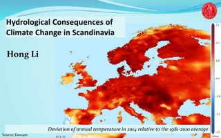
  • 1. Hong Li Deviation of annual temperature in 2014 relative to the 1981-2010 average Source: Euro4m
  • 2. Outline 2  Global Climate Change  Methods  Climate Change in Scandinavia • Temperature • Precipitation (Extreme & Snow)  Hydrological Consequence • Runoff • Glaciers
  • 3. Climate 3 Climate describes the average weather over a certain time-span (usually 30-year period) in a certain location.
  • 4. Climate Change 4 Statistically significant variations of the mean or variability, typically persisting for decades or longer. Temperature, wind, precipitation, humidity, cloud, radiation Source: IPCC AR3
  • 5. Global Climate Change 5Data source: NOAA Global average temperature anomalies 1880 – 2014 1965 – 2014 0.26/decade 0.16/decade 0.12/decade
  • 6. Changes in annual temperature between 2000 – 2014 and 1961 – 1990 6Source: NASA Global Climate Change Zonal mean changes against latitude
  • 7. Global Climate Change 7 Energy Balance of the Earth Source: Zolushka, 2015 CO2
  • 8. Global Climate Change 8 Reconstructed temperature anomalies (°C) relative to present from Vostok and EPICA Source: ClimateData ‘Milankovitch cycle‘, the changes in the way the earth orbits the sun
  • 9. 9 Source: USGCRP, 2009; IPCC AR5 Concentraion of 3 green house gases Global Climate Change Global land surface temperature anomalies relative to 1880 – 1919 Observations With human emissions Without human emissions 1 °C
  • 10. Global Climate Change 10 Less Sea Ice Source: EPA January 2014 Norway August 2014 Sweden
  • 11. Outline 11  Global Climate Change  Methods  Climate Change in Scandinavia • Temperature • Precipitation (Extreme & Snow)  Hydrological Consequence • Runoff • Glaciers
  • 12. Methods Signal Trend Detection • Linear trend • Mann-Kendall Test + Sen slope Future Climate and Impacts • (AO)GCMs • RCMs • Bias Correction/Downscaling • Hydrological Models (HM) 12 AOGCMs: Atmosphere–Ocean General Circulation Models RCMs: Regional Climate Models 𝑋 = 𝑎 × 𝑌𝑒𝑎𝑟 + 𝑏
  • 13. Methods Future Climate and Impacts • (AO)GCMs • RCMs • Bias Correction/Downscaling • Hydrological Models (HM) 13 Source: Bice, 2015 10-20 layers 20 layers 100 – 600 km
  • 14. Methods 14Source: ConsulClima Future Climate and Impacts • (AO)GCMs • RCMs • Bias Correction/Downscaling • Hydrological Models (HM)
  • 15. 𝑆𝑀𝑒𝑙𝑡 = 𝑆𝑀𝐸𝐿𝑇𝑅 × 𝑻 − 𝑇𝑚𝑒𝑙𝑡 𝐼𝑀𝑒𝑙𝑡 = 𝐼𝑀𝐸𝐿𝑇𝑅 × (𝑻 − 𝑇𝑚𝑒𝑙𝑡) P 𝐸 = 𝐸𝑃𝑂𝑇 × 𝑻 𝐴𝐸 = 𝑃𝐸 𝑃𝐸 × 𝑆𝑀 𝐹𝐶 𝐹𝐶𝐷 𝑄0 = 𝐾𝑈𝑍 × 𝑈𝑍 𝛼 𝑄1 = 𝐾𝐿𝑍 × 𝐿𝑍 15 Scheme of the HBV model Methods
  • 16. Methods Advantages • 4-D global scale simulation • More climate components • Finer description of processes • Increasing resolutions 16 Source: IPCC AR4
  • 17. Methods Disadvantages • Simpler than reality: teleconnections • Too sparse scales for local processes: extreme events • Limitations in chemistry and interactions 17 Source: Lupo et al., 2013 Good: fluid motions of atmosphere and oceans Poor: clouds, dust, chemistry, biology Good: Temperature Poor: Precipitation
  • 18. Outline 18  Global Climate Change  Methods  Climate Change in Scandinavia • Temperature • Precipitation (Extreme & Snow)  Hydrological Consequence • Runoff • Glaciers
  • 19. 19 Sweden 450,295 km2; 4.7⁰C/643 mm Norway 323,802 km2; 1.0⁰C /1104 mm Denmark 43,094 km2; 7.7⁰C/712 mm Climate Change in Scandinavia 1961 – 1990 AnnT/AnnP
  • 20. Fast warming • 0.26 °C/decade Global Land • 0.37 °C/decade in Norway • 0.36 °C/decade in Sweden (a) (b) (c) Source: Drange, 2015; SMHI; DMI Temperature 20 (a) Norway (relative to 1901 – 2000 mean) (b) Sweden (relative to 1961 – 1990 mean) (c) Denmark -/0.36 °C/decade
  • 21. Temperature 21 Seasonal difference • More increase in Winter • Less increase in Summer Source: Nilsen, 2015 Monthly temperature changes over the 31-year periods for mainland Norway Temperaturechange(°C)
  • 22. Temperature 22 Spatial variation • More increase in North • Less increase in South Temperature trend (°C/decade) in January Watch Forcing Data ERA-Interim 1979 – 2009 Source: Irene, 2015
  • 23. Temperature 23 Temperature change (°C) in 2071 – 2100 relative to 1971 – 2000 by 9 GCMs, RCA4, Rcp8.5 Source: SMHI Annual Winter Summer
  • 24. More precipitation • 18/31% per 100 yr in Norway • 17/34% per 100 yr in Sweden 24 (a) (b) (c) Source: Drange, 2015; SMHI, DMI Precipitation (a) Norway (relative to 1901 – 2000 mean) (b) Sweden (c) Denmark 17/34 % per 100 yr
  • 25. Precipitation 25 Seasonal difference • More increase in winter and less in summer Source: Drange, 2015 Change in precipitation in Norway (relative to 1901 – 2000) (a) winter (b) summerWinter Summer
  • 26. Relative increase in annual precipitation 1990 – 2003 to 1961 – 1990 Spatial variation • More increase in North and West Norway. Precipitation 26Source: : Thorsteinsson & Björnsson, 2011
  • 27. Precipitation 27 Annual Winter Summer Relative change (%) in 2071 – 2100 to 1971 – 2000 by 9 GCMs, RCA4, Rcp8.5 Source: SMHI
  • 28. Precipitation: Extreme Yearly Maximum 1 day 28 Mean of yearly maximum precipitation (bars) based on 60 long- term stations in Sweden. Red curve is smoothed value. Dotted black curve smoothed value based on 740 stations. Trend (% per decade) in 1900 – 2004 relative to 1961 – 1990 Source: SMHI; Alfnes & Førland, 2006
  • 29. Precipitation: Extreme 29 Sub-daily Relative change in 10-year rainfall amount (1981 – 2010) averaged over Sweden in the projections. Vertical line represents ± one standard deviation. Grey symbol represents a change that is not statistically significant. 2011 – 2040 2071 – 2100 Source: Olsson & Foster, 2014
  • 30. Precipitation: Snow Less snow days 30Source: Dyrrdal, 2009 Linear trend in No. of snow days for all observations 10 statistically positive (low temperature) 247 statistically negative Stronger in southeast and southern coast Stronger after 1990 No./year
  • 31. Precipitation: Snow Less snow depth 31Source: Dyrrdal, 2009 No. of snow days Annual mean depth (cm) Max. 1-d increase (cm) Tunnsjø Location: (13.6506, 64.6837) Height: 376 masl 1.9 days/decade
  • 32. Precipitation: Snow Less snow in the future 32 Relative change (2071 – 2100 to 1961 – 1990) By HIRHAM, Hadley, B2 Echam show similar results altitude distance from the coast. Source: Vikhamar-Schuler & Førland, 2006
  • 33. Precipitation: Snow Less snow in the future 33 Relative change (2071 – 2100 to 1961 – 1990) By HBV driven by HIRHAM, Hadley, B2 Echam show similar results Source: Vikhamar-Schuler & Førland, 2006
  • 34. Precipitation: Snow Different between RCM and HM 34 Relative change in SWE 2071 – 2100 to 1961 – 1990 By HBV and HIRHAM Hadley, B2 HBV HIRHAM Below 200 masl 200-1000 masl Above 1000 masl Source: Vikhamar-Schuler & Førland, 2006
  • 35. Outline 35  Global Climate Change  Methods  Climate Change in Scandinavia • Temperature (increase) • Precipitation (increase but less Snow)  Hydrological Consequence • Runoff • Glaciers Water resources, hydropower potential Limitations of the hydrological models Flood
  • 36. Runoff 36 Trends in annual runoff (1961 – 2000) Source: Wilson et al., 2010 Increase at 95%significance level Increase at 70%significance level No trend Decrease at 70% significance level Decrease at 95% significance level Observed annual increase
  • 37. Runoff 37 Relative increase in annual runoff 1990 – 2003 to 1961 – 1990 Source: Thorsteinsson & Björnsson., 2011 Observed annual increase
  • 38. Runoff 38 Annual runoff Source: Thorsteinsson & Björnsson., 2011 Annual precipitation
  • 39. Runoff 39 More runoff in future Change in seasonality Source: JesF, 2007 Daily mean discharge in 2071 – 2100 by four precitions
  • 40. Source: Beldring et al, 2006 Runoff 40 Annual Winter Spring
  • 41. Source: Beldring et al, 2006 Runoff 41 Spring Summer Autumn
  • 42. Runoff 42 Season of annual Max. runoff 25 HBV best parameter sets 8 GCMs, 5RCMs, A2, B2, A1B Change in flood time Source: Lawrence & Hisdal, 2011
  • 43. Runoff 43 Change in flood magnitude Median change of the change for the 100-year flood in Sweden (%) 2021 – 2050 to 1963 – 1992 Based on 16 regional climate scenarios Distribution Based Scaling (DBS) approach 1001 river basins. Source: Thorsteinsson & Björnsson, 2011 Lawrence & Hisdal, 2011 shows similar results in Norway
  • 44. Runoff 44 Change in flood magnitude Tora, 263 km2 700 – 2014 masl North-western In southern Norway HBV, HIRHAM5, ECHAM5, A1B HBV, HIRHAM, HadCM3, A1B HBV, RCA3, BCM, A1B 100-year flood based on 30-year moving data Source: Thorsteinsson & Björnsson, 2011
  • 45. Runoff: Glaciers 45 1960 1970 1980 1990 2000 2010 -3 -2 -1 0 1 2 3 Time (yr) Massbalance(mw.e.yr -1 ) Winter Annual Summer Glacier mass balance of mainland Norway +1.92 -0.86 -2.78 Source : Engelhardt et al, 2013; Zemp et al, 2010 Cumulative specific mass balance of Storglaciären. -0.4 m w.e. yr-1
  • 46. Runoff: Glaciers 46 coupled mass balance/ice-dynamic or mass-balance/glacier-scaling models various GCMs, RCMs, A1B Source: Thorsteinsson & Björnsson, 2011
  • 47. 47 Negative Effects • Disturb biodiversity • Affect landscape and tourism Reasons • Regrowth • Climate change Interactions Source: Rübberdt; Bryn & Hemsing, 2012; Bryn, 2008 24.6 million m3 per year in 2007 – 2011 in Norway
  • 48. 48 Evaporation and cloud • Heat flux • Water vapour • Increase reflection Absorb carbon Reduce albedo Interactions Source: DeWit et al, 2014
  • 49. Summary  Temperature • Has increased more than 0.35°C/decade in Norway and Sweden (1965 – 2014) • Will very likely amplify in future (more than 0.5°C/decade Rcp8.5) Precipitation • Has increased more than 30% in Norway and Sweden (1965 – 2014) • Will likely increase in the future and less snow Runoff • Has increased and will continue with more glacier melting • Large spatial variations and change in seasonality 49

Editor's Notes

  1. Thank you for the introduction and Welcome you all to my trail lecture about ‘Hydrological Consequences of Climate Change in Scandinavia’. Here shows a map of the deviation of annual temperature in 2014 relative to the 1981-2010 average. Last year was the hottest year on Earth and also in Europe.
  2. In total, there are four parts. First, I will give a global picture about climate change and the global effects. Then I will introduce the common used methods. In the third part, I will show the climate change in Scandinavia, mainly about temperature and precipitation. As affected by climate, I will show the changes in runoff and glaciers. First, let’s see two definitions, climate and climate change.
  3. Climate describes the average weather over a certain time-span (usually 30-year period) in a certain location. It is different from weather.
  4. Climate change means statistically significant variations of the mean or variability, typically persisting for decades or longer. The changes can be in mean and variance, and leads to different effects. We mainly concern the parameters affect daily life, such as temperature, wind, precipitation, humidity and so on. Temperature and precipitation are the most important parameters to hydrology; therefore, I will focus on temperature and precipitation.
  5. Temperature is the first indicator of climate change. Here shows the global average temperature since 1880 to 2014. There is a significant warming trend, particularly after the 1980s. For last 50 years, from 1965-2014, the slope is 0.26 centigrade per decade for land, 0.16 for average and 0.12 for ocean.
  6. The warming is not evenly distributed. Warming is much stronger in Norther Hemisphere than South Hemisphere. The artic is four times of the equator area. This is called ‘amplifier effects’.
  7. The surface temperature is determined by the earth internal processes and out forcing. The Sun is the source of energy. The total solar radiation is around 342 watt per square meters. However, only 47% can be absorbed by the earth. The remaining is absorbed by the cloud or reflected back to the space. At the same time, the atmosphere and the earth also emit longwave radiation. A large part of the atmosphere radiation is towards the earth surface, warming it. Putting a lot of CO2 or other greenhouse gases into the atmosphere will increase the longwave radiation to the earth surface. Let’s see their individual effects.
  8. This figure shows two reconstructed temperature series back to 450 thousand years ago. The two stations are located in the east Antarctica. They show that earth has gone through several warm and cold cycles. The highest was about five centigrade higher than now. We are currently in a warming period and have not reached previous peak values. Most of the variations can be explained by ‘Milankovitch cycles’, in the way the earth orbits the sun.
  9. The concentrations of three greenhouse gases have significantly increased. Since 1750, the increase is due to human activities in the industrial era. CO2 has the highest concentration and is the main greenhouse gas. The impacts are given by run climate models with human emissions and without human emissions. I will talk about climate models later. The black line is the observed global land surface temperature relative to 1880 to 1919. The results with human emissions match quite well with observations. It is 1 centigrade warmer than without human emissions. As state in the IPCC fifth assessment report, it is extremely likely that half of the warming is caused by greenhouse gas and half of the emission is caused by human activities.
  10. Climate change has important impacts on many aspects of the nature. Observations have confirmed the predictions. For example, higher temperature and more heat waves, less snow and ice, rising sea level. The predictions by climate models have higher confidence. These are extreme likely to happen in future. Some others items, for example, change in rain and storms, drought, indeed has confirmed by observations. There are more forest fires to occurred in the previously unlike seasons. For example, January and August, last year. The changes also feedback to the climate system, making the accurate predictions difficult. Some plants are growing and will be a carbon sink. Thawing permafrost will release more greenhouse gases and further warm the climate. The changes are not uniformly distributed. The rising sea level rise will pose high pressure for mid-latitude and low latitude areas. However, for Norway and Sweden, the absolute sea level is rising, But due to the land uplift, the net sea level or relative sea level is getting lower.
  11. I have talked about the first part global climate change. The second part is the methods, how to make climate predictions and study it impacts.
  12. The methods can be divided into two groups. The first group is climate signal trend detection. They are used to analyse the observed data to determine if the changes are significant and how much. The most used significant is Mann-Kendall test. Linear regression is the simplest method to determine the magnitude of change, the parameter a. It can be in absolute or relative. For the future, generally, there are four steps.
  13. The first step is to generate future climate. The general circulation models represent physical processes in the atmosphere, ocean, cryosphere and land surface. They are widely used for daily weather prediction. They typically have a horizontal resolution of between 250 and 600 km, 10 to 20 vertical layers in the atmosphere and sometimes as many as 30 layers in the oceans.
  14. The resolution is too large for regional study. The results are future downscaled by regional climate model, the resolution is typically 50 kilometers. The results can be future downscaled to the observe locations. This technique is also called bias correction. Eventually, the results are inputs to hydrological models. The hydrological models will produce the runoff series considering the vegetation, soil and topography.
  15. This is a typical conceptual hydrological model, the HBV model. It was initially developed for the Scandivinia conditions in the 1970s. Now it has been applied in more than 80 countries, particularly in North Europe. The inputs are precipitation and temperature. Melting of snow and ice is a degree-day method. Evaporation is based on temperature and soil moisture. Runoff dynamics is simulated two ground reservoirs. The parameters values can be calibrated or derived from soil and vegetation data.
  16. I have introduced general methods. For the future, the impact studies are mainly based on GCMs, RCMs and hydrological models. Large uncertainties can be caused by each kind of models. Their outputs should be examined carefully and cautiously. There, I want to highlight the advantages and disadvantages of GCMs, which is less discussed. The GCMs are the most advanced and complex available tools. They can provide four dimension global scale simulation. The models become more complex from the IPCC first assessment to the forth report. More processes are included. The resolutions are also increasing.
  17. However, we should also know their disadvantages. This is where to improve and make them better. First, the models are complex, but still simpler than the reality. For example, teleconnections play an important role in climate variations, but the models cannot predict them. Second, the spatial resolutions are too sparse, particularly for prediction in extreme events. They usually happen in a short time and a small area. Third, the models are still quite poor in chemistry and interactions. For process, they do a very good job of describing the fluid motions of the atmosphere and the oceans. They do a very poor job of describing the clouds, the dust, the chemistry and the biology. More closely to hydrology, the model can predict good temperature but more inaccuracy in precipitation.
  18. I have briefly introduced the methods. For future, the general procedures are running GCMs, RCMs, bias correction and then hydrological models. It is also important to know that the models are reliable in temperature, but less confidence in precipitation. The next part is climate change in Scandinavia. I will focus on temperature and precipitation.
  19. Scandinavia is controversial word. There I pick the definition from Wikipedia. Scandinavia is a historical region in Northern Europe. There are three countries, Sweden, Norway and Denmark. They share similar culture and language. Officially people speak three different languages, but people adapt to each other very quickly and use the same Scandinavia language and English. The annual air temperature and annual precipitation is calculated for the period 1961 to 1990, usually used a reference period in climate change studies. Among the three countries, Sweden is the largest and dries. Norway is the coldest and has the highest precipitation. Denmark is very small, less than ten percent of Sweden. Its climate is more similar to the West Germany. So I will give climate information about Denmark, but more focus on Sweden and Norway.
  20. The three figures show the annual temperature of Norway, Sweden and Denmark. All of them show an increasing trend, similar as the global average. For the last 50 years, the trend of global land is 0.26 centigrade per decade. For the same period, the trend for Norway is 0.37 and 0.36 for Sweden. This is a much faster than the global average. Additionally, there are some regional variations. For example, the period during the 1930s and 1940s was quite warm in the tree countries, but it was not a globally warm period. Another example is 2010. It was a cold year, but a global warm year.
  21. The warm trends have very significant seasonal differences. This figure shows monthly temperature change for three periods for the mainland Norway. The blue line is for 1959 to 1989, dashed line is for 1969 to 1999 and red line is for 1979 to 2009. We can see that the temperature change is accelerating. Additionally, within a period, there is more increase in winter than in summer. This seasonal difference will have significant impacts on snow and runoff.
  22. The change is not spatially uniform. This map shows the temperature trend in January from 1979 to 2009. Generally, the North is redder that the South, which means a higher trend. Besides, the black dots indicate significant at 95% level. The trend in the North is significant.
  23. For the future, predictions for 2071 to 2010 show that temperature will continue increase. This maps are produced by 9 GCMs, RCA4, which is a regional climate model, under the emission scenario Rcp8.5. They show that the warming will continue. The change in annual temperature is between three and seven, increasing from South to North. Similar as the observations, more increase in winter than in summer. In winter in North, the change can be up to 10 centigrade.
  24. Precipitation also show positive trend. The three figures show the annual precipitation for Norway, Sweden and Denmark. The increase is accelerating. For the last 100 years, the trend is 1.8% in Norway; for the last 50 years, the trend is 31% per 100 yr. The values are 17% and 34% in Sweden. Research by the Norwegian Meteorological Institute shows the change is partly due to change in circulation.
  25. The change in precipitation also shows seasonal difference. The change in winter is significantly more than in summer. For the last 50 years, the trend in winter is 58% per 100 yr, and it is 36% in summer.
  26. Here gives the spatial variation in annual precipitation in 1990 to 2003 based on 1961 to 1990. The largest increase happened in North and West coast, almost 6 percent. The southern-east increased the lest, only 1.5 percent.
  27. In the future, the precipitation will continue to increase, more than 20% in 2071 to 2100. Generally, there will be more in North than South. However, the spatial pattern is a bit confusing. This may be caused by less confidence of GCMs in precipitation than temperature. The spatial resolution, 55 km is too large.
  28. Additional to the annual and season precipitation, extreme events are also very important. They likely cause flash flood, which is difficult to predict. Here I will analyses the yearly maximum 1 day precipitation. This figure shows the mean of 60 long terms stations since 1900. Red shows the smoothed values of the bars. The values fluctuates between 30 to 40 mm. since 1990s, there is slightly increasing trend, roughly from 32 mm to 35 mm. The red dotted line show values based on all available stations, 740. They show the same variation with higher values. That is caused by locations of the stations. The 740 stations include a relatively large proportion of inland stations, which generally measure greater precipitation than coastal stations. Let us look at a station level and how much is it. Most station have a small increasing trend, but not significant. Only four stations are significant. Predictions by the same project show the maximum 1 day is not likely to increase before 2050, but likely to increase in long term.
  29. In next 30 years, change is small, increase with small duration as well as the uncertainty. Small models even predict negative change. For the end of the century, all models predict positive.
  30. Snow is important in our daily life and hydropower predictions. There is a general decrease in the number of snow days in the entire country. Only 10 stations reveal statistically significant positive trends at the 95 % confidence level, compared to 247 statistically significant negative trends. Temperature of the positive stations is very low in the winter. Spatially, there is a stronger tendency in the southeast and along the southern coast. The negative trend is steeper from 1990 until the end of date, 2009.
  31. Another station is located near the border of Norway and Sweden. It elevation is 376 meter above sea level. In this area, there are many reservoirs and hydropower stations. So I also plot its annual mean depth in snow water equivalent. The trend is 1.9 days per decade, much less than other two stations. For annual depth, there is a small negative trend. However, the maximum 1 day increase, indicating maximum the snowfall amount in one day, shows a positive trend. This indicates that intensified snowfall and fast melting.
  32. The future can be predicted by regional climate model and hydrological models. The snow water equivalent is predicted to decrease almost everywhere in three countries in 2017 to 2100 by the GCM Hadley under B2 scenario. Another GCM Echam show similar results. Generally, the changes get smaller with altitude and distance to coast.
  33. Further they used the precipitation and temperature from the regional climate model to drive the HBV model. The HBV model was run in 1 km spatial resolution. It is a very fine resolution compared to the RCM resolution, 55 km. The HBV model generated a similar pattern as the Regional climate model. But with higher resolution, the HBV model has large variability, particularly in south-west coast and inland high elevation. The HBV gave positive change in some area. It is also possible because at the very high mountains, the temperature will still quite low. With more precipitation, the snow storage will increase.
  34. To find the systematic pattern, the grids are divided into three groups, below 200 m by close circle, 200 to 1000 m by open circle and above 1000 m by cross. The two ways estimate similar relative changes in areas located below 200 m. In the areas above 1000 m, the HBV model estimates less change than the HIRHAM model.
  35. I have showed about the observed and predicted change in temperature and precipitation. Here I want to make a small summary. The temperature has increased. The climate models predict that the increase will amplify in the future. At the same time, the precipitation also increases. Due to high temperature, snow becomes less. These changes have very important impacts on runoff. I will show the runoff and glaciers. Runoff is used as criteria of water resources and hydropower potential. As an indicator of the risk, I will talk about flood. Due to the fact that current hydrological models cannot well simulate glaciers and they are very important in the hydrological system. So I will additionally talk about glaciers.
  36. In the period of 1961 to 2000, there is an increase in annual runoff in three countries. In this map, the blue circles indicate significant positive at 95% confidence level. Light blue indicates significant positive at 70% confidence level. There are only two stations show weak negative trend, one in Norway and one in Finland. Most of the significant positive stations are located in the North Sweden or West coast of Norway.
  37. This map shows how much the runoff has increase in 1990 to 2003 compare to 1961 to 1990. The largest increase happened in North Norway, more than 9 percent. The least is in the south-east Norway, only 0.1 percent.
  38. If we compare the annual precipitation change in the same period, as I have shown in precipitation, there are two regions that runoff increase more than precipitation, the North and south-west mountain areas. In these two areas, there are some glaciers and limited energy in evaporation.
  39. In future, the runoff is predicted to increase both in Norway and Sweden. The figure shows four predictions in 2071 to 2100. The change in Norway is much larger than in Sweden. In both countries, all predictions show less summer runoff and more winter runoff. In Sweden, the maximum discharge is predicted much earlier. In Norway, two predictions even indicate the maximum discharge will change into autumn. It is very likely that there will be more runoff and the seasonality will change. But for the magnitude, there are quite large spreads. In Norway, predictions of the dark blue are suspect to unlikely.
  40. These maps show the spatial pattern in 2071 to 2100 compared to 1961 to 1990. Blue indicates increase and red indicates decrease. For annual runoff, most places will increase between 5 to 20 percent. The largest decrease will happen in south east Sweden. The magnitude is more than 75% percent. The winter runoff will increase. The spring runoff has the largest variations. In the coast area, spring runoff is going to decrease, in the inland area, it is going to increase.
  41. These maps show the summer runoff and autumn runoff. The summer runoff is going to decrease almost everywhere. The reasons are increased evaporation and less snow storage. The autumn runoff is decrease in south but increase in north.
  42. As a change in the seasonality, the maximum discharge will change from summer to spring.
  43. The 100-year flood was used as the common basis for comparing results based on flood frequency analysis. This figure shows the median change for the 100-year flood in Sweden (%) from the period 1963–1992 until the period 2021–2050. The results are based on 16 regional climate scenarios and the Distribution Based Scaling (DBS) approach in 1001 river basins. The 100 year change more or less, but most areas are within in the positive or negative 15% range. It is likely that in the near future, the 100 year flood does not change. It is the same as Norway.
  44. What about in long term and how reliable the results are. Here I select a small catchment in North-western Mountain in southern Norway. The Tora catchment is 263 suqre kilometers, the elevation range is 600 to 2014 meter. The figure shows the estimated 100 year flood based on 30 years data by three predictions. The discharge is generated by HBV model, but different regional climates and GCMs, under A1B emission scenario. There is large spread among the models, but at the end of century, the 100-year is much higher than 1961 to 1990.
  45. The glaciers in Scandinavia are relative small in the world, but they are very important in hydro-power productions. This figure shows the glacier mass balance of mainland Norway. Before 1990, the annual mass balance fluctuated around zero. The mass balance was negative afterward and the rate was accelerating after 2000. From 2000 to 2010, the annual mass balance is -0.86 meter per year, caused by less winter accumulation and more summer melting. The Swedish glaciers are also in negative mass balance. This figure shows the accumulative specific mass balance of storglacier by different studies. It has the longest record in Norway and Sweden. In period of 1975 and 1985, the glacier was in a balanced situation. However, after 1995, the annual mass balance is -0.4 meter per year. The green dashed line includes the internal accumulation. It can be caused by the refreezing of surface melt. The surface elevation is decreased, but the total mass does not change, since the water refreeze in the glacier. In 1995, the internal accumulation was around 2 meters, but does not change mass balance after 1995.
  46. The glaciers in Norway and Sweden are predicted to continuously decrease. This figure show the predicted volume by various glacier mass balance, dynamics models driven by many GCMs, RCMs under A1B scenario. There are three glacier in Iceland, three glacier in Norway and two glacier in Sweden. All glaciers are predicted shrink in the future. For example, at the end of century, the Midaltsbreen and Nigardsbreenn will be only 20 percent of the 2000 volume.
  47. All these prediction do not account the interaction of the landscape to climate, or called feedback. Sometimes, the feedback can be very significant to the climate. For example, it has been observed that Extensive forest expansion has taken place across Europe during recent decades. It is also a major trend in Norway, with an annual increase of about 24.6 million m3 during 2007–2011. Open landscapes are likely to become more quickly overgrown by shrubs and trees. This expansion is usually describe as negative, since the disturb biodiversity and making paths less accessible and blocking views. Research has shown that this expansion is mainly regrowth. Since farm is abandoned and sheep grazing is less. This area is growing to forest again. However, in some small areas, the trees start to grow above tree line. This is mainly caused by climate change.
  48. However, this growth has complex effects on climate. With more vegetation, there will be more evaporation, taking more heat to the atmosphere and increase the water vapor content. However, the water vapor is a very stronger greenhouse gas, will warm the climate. At the same time, more cloud will increase reflection and reduce the solar radiation, cool the climate. The vegetation will absorb carbon and reduce the albedo. If only consider the vegetation carbon and albedo, the warm effects can be up to 10 times of cool effect in south western Norway.
  49. To summaries, the temperature has increase and will continue. The precipitation has increase and will continue and less snow. Runoff will increase but with large variation and more glacier melting. All the changes are more in North than in South.