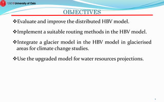
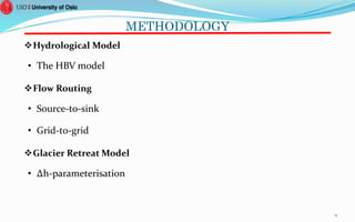
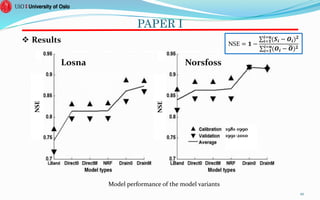
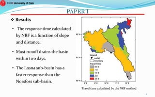
SlideShare a Scribd company logo
Ph.D. Dissertation presented by
Hong Li
Chongyu Xu (UiO); Stein Beldring (NVE); Lena Tallaksen (UiO)
OUTLINE
 Part I
• Motivation & Objectives
• Study Area & Data
• Methodology
 Part II
• Paper I: Li, H. et al., 2014. Implementation and testing of routing algorithms in the distributed HBV model for mountainous
catchments. Hydrology Research, 45(3), pp.322–333.
• Paper II: Li, H. et al., 2015. How much can we gain with increasing model complexity with the same model concepts? Journal of
Hydrology, 527, pp.858–871.
• Paper III: Li, H. et al., 2015. Integrating a glacier retreat model into a hydrological model – Case studies of three glacierised
catchments in Norway and Himalayan region. Journal of Hydrology, 527, pp.656–667.
• Paper IV: Li, H. et al., 2015. Water Resources under Climate Change of Himalayan Basins. Water Resources Management,
submitted.
Publications
2
MOTIVATION
Hydrological models are important tools for climate change
impact studies.
Distributed hydrological models are prevalent in research
but not widely used in operational hydrology.
Glaciers are very sensitive to climate change and they have
affected the regional hydrological regime, but few
hydrological models can reproduce glacier processes.
Reliable water resources projections are essential to society
development.
3
OBJECTIVES
Evaluate and improve the distributed HBV model.
Implement a suitable routing methods in the HBV model.
Integrate a glacier model in the HBV model in glacierised
areas for climate change studies.
Use the upgraded model for water resources projections.
4
STUDY AREA & DATA
 Four basins are used
• Glomma Basin in Norway
• Nigardsbreen Basin in Norway
• Beas Basin in India
• Chamkhar Chhu Basin in Bhutan
5
STUDY AREA & DATA—Glomma Basin
 Glomma Basin
• 41,963 km2; ~15 % of Norway
• P: 720 mm/year; T: 2.9 ◦C
 Losna Sub-basin
• 11,213 km2; 1158 m amsl; 11.8◦
 Norsfoss Sub-basin
• 18,923 km2; 732 m amsl; 6.7◦
6
Location of the Glomma Basin
STUDY AREA & DATA—Glomma Basin
Norsfoss Sub-basin
• 18,923 km2; 732 m amsl; 6.7◦
• 7 discharge stations
• 3 snow pillows
• 7 groundwater piezometers
7
Locations of stations in the Norsfoss Basin
STUDY AREA & DATA—Nigardsbreen Basin
 Nigardsbreen Basin
• The Nigardsbreen station
• Western Norway
• 65 km2;
• P: 3736 mm/year; T: -0.47 ◦C
• 72.8% covered by glaciers
8
Map of the Nigardsbreen Basin
STUDY AREA & DATA—Himalayan Basins
 Beas Basin
• The Bhuntar station
• Northern India
• 3202 km2;
• P: 1116 mm/year; T: -1.04 ◦C
• 32.7% covered by glaciers
9
Map of the Beas Basin
STUDY AREA & DATA—Himalayan Basins
 Chamkhar Chhu Basin
• The Kurjey station
• Central Bhutan
• 1353 km2;
• P: 1786 mm/year; T: 1.75 ◦C
• 15.0% covered by glaciers
10
Map of the Chamkhar Chhu Basin
METHODOLOGY
Hydrological Model
• The HBV model
Flow Routing
• Source-to-sink
• Grid-to-grid
Glacier Retreat Model
• Δh-parameterisation
11
METHODOLOGY—Hydrological Model
𝑆𝑀𝑒𝑙𝑡 = 𝑆𝑀𝐸𝐿𝑇𝑅 × 𝑇 − 𝑇𝑚𝑒𝑙𝑡
𝐼𝑀𝑒𝑙𝑡 = 𝐼𝑀𝐸𝐿𝑇𝑅 × (𝑇 − 𝑇𝑚𝑒𝑙𝑡)
P 𝐸 = 𝐸𝑃𝑂𝑇 × 𝑇
𝐴𝐸 =
𝑃𝐸
𝑃𝐸 × 𝑆𝑀 𝐹𝐶 𝐹𝐶𝐷
𝑄0 = 𝐾𝑈𝑍 × 𝑈𝑍 𝛼
𝑄1 = 𝐾𝐿𝑍 × 𝐿𝑍
12
Scheme of the HBV model
METHODOLOGY—Flow Routing
Flow Routing
13
Sub-Basin
Junction
Channel
Outlet
Element-to-Element
Outlet
Source-to-Sink
Land
Outlet
Grid-to-Grid
Land
METHODOLOGY—Flow Routing
Flow Routing
• Source-to-sink
Network Response Function: 𝑡 = 𝑖=1
𝑖=𝑛 𝑙 𝑖
𝑉45× tan 𝑆𝑖
• Grid-to-grid
Hillslope routing: 𝑆𝑀𝑗= 𝑁𝑒𝑡𝑃𝑗 + 𝑖=1
𝑖=𝑛
𝑅𝑖
Channel routing : Muskingum-Cunge method
14
𝑆𝑀: 𝑠𝑜𝑖𝑙 𝑚𝑜𝑖𝑠𝑡𝑢𝑟𝑒; 𝑁𝑒𝑡𝑃: 𝑛𝑒𝑡 𝑝𝑟𝑒𝑐𝑖𝑝𝑖𝑡𝑎𝑡𝑖𝑜𝑛; 𝑅: 𝑟𝑢𝑛𝑜𝑓𝑓
𝑡: 𝑡𝑖𝑚𝑒; 𝑙: 𝑙𝑒𝑛𝑔𝑡ℎ; 𝑉45: 𝑣𝑒𝑙𝑜𝑐𝑖𝑡𝑦 𝑝𝑎𝑟𝑎𝑚𝑒𝑡𝑒𝑟; 𝑆𝑖: 𝑠𝑙𝑜𝑝𝑒
METHODOLOGY—Glacier Retreat Model
∆𝒉 = 𝒉 𝒓 + 𝒂 𝜸
+ 𝒃 × 𝒉 𝒓 + 𝒂 + 𝒄
𝒉 𝟏 = 𝒉 𝟎 + 𝒇 𝒔 × ∆𝒉𝒊
15
Scheme of the Δh model
𝑩 𝒂 = 𝒇 𝒔 × 𝝆𝒊𝒄𝒆 ×
𝒊=𝟏
𝒊=𝒏
𝑨𝒊 × ∆𝒉𝒊HBV
Huss et al. 2010
OUTLINE
 Part I
• Motivation & Objectives
• Study Area & Data
• Methodology
 Part II
• Paper I: Li, H. et al., 2014. Implementation and testing of routing algorithms in the distributed HBV model for mountainous
catchments. Hydrology Research, 45(3), pp.322–333.
• Paper II: Li, H. et al., 2015. How much can we gain with increasing model complexity with the same model concepts? Journal of
Hydrology, 527, pp.858–871.
• Paper III: Li, H. et al., 2015. Integrating a glacier retreat model into a hydrological model – Case studies of three glacierised
catchments in Norway and Himalayan region. Journal of Hydrology, 527, pp.656–667.
• Paper IV: Li, H. et al., 2015. Water Resources under Climate Change of Himalayan Basins. Water Resources Management,
submitted.
Publications
16
PAPER I
17
PAPER I
Objectives
• Compare the routing methods in the Norwegian context.
• Improve the HBV model by implementing routing function.
• Obtain a complete distributed HBV model.
18
PAPER I
 Methods: 6 model variants
• LBand: semi-distributed model with elevation bands
• Direct0: grid-based model; no routing
• DirectM: grid-based model; Muskingum-Cunge
• NRF: grid-based model; source-to-sink method
• Drain0: grid-based model; hillslope routing
• DrainM: grid-based model
hillslope routing and Muskingum-Cunge
19
PAPER I
 Results
20
Losna Norsfoss
Model performance of the model variants
1981-1990
1991-2010
NSE = 𝟏 −
𝒊=𝟏
𝒊=𝒏
(𝑺𝒊 − 𝑶𝒊) 𝟐
𝒊=𝟏
𝒊=𝒏
(𝑶𝒊 − 𝑶) 𝟐
NSE
NSE
PAPER I
21
Travel time calculated by the NRF method
 Results
• The response time calculated
by NRF is a function of slope
and distance.
• Most runoff drains the basin
within two days.
• The Losna sub-basin has a
faster response than the
Norsfoss sub-basin.
PAPER I
 Conclusions
• Grid-based models are better than the semi-distributed model.
• The routing methods improve the grid-based models.
• The hillslope routing makes the most significant improvements.
22
PAPER II
23
PAPER II
Objectives
• Examine the model performance more deeply by including interior
points and internal variables.
• Does higher model complexity lead to better performance?
• Investigate effects of spatial discretisation and process description on
model performance.
24
 Methods: 5 model variants
• LWhole: lumped model
• SBand: semi-distributed with elevation bands
• GRZero: grid-based model; no routing
• GROne: grid-based model; hillslope routing
• GRTwo: grid-based model; hillslope and channel routing
PAPER II
25
PAPER II
 Results: Runoff
26
Monthly mean runoff simulations by the five model variants.
PAPER II
 Results: Runoff
27
-0.2
0
0.2
0.4
0.6
0.8
1
158 377 463 550 1646 15447 18933
NSE
Area (km2)
Average
LWhole
SBand
GRZero
GROne
GRTwo
Model performance at all discharge stations
𝑵𝑺𝑬 = 𝟏 −
𝒊=𝟏
𝒊=𝒏
(𝑺𝒊 − 𝑶𝒊) 𝟐
𝒊=𝟏
𝒊=𝒏
(𝑶𝒊 − 𝑶) 𝟐
PAPER II
 Results: groundwater
28
Model performance at three grid-based models in simulating groundwater measurements
R= 𝒊=𝟏
𝒊=𝒏
𝑶 𝒊− 𝑶 𝑺 𝒊− 𝑺
𝒊=𝟏
𝒊=𝒏 𝑶 𝒊− 𝑶 𝟐
𝒊=𝟏
𝒊=𝒏 𝑺 𝒊− 𝑺 𝟐
PAPER II
 Conclusions
• The model performance in runoff simulation improve with more
complexity, particularly in the low flow.
• The model performance at the interior points increases with larger
area.
• The models are similar in reproducing the internal variables, such as
evaporation, snow and groundwater.
29
PAPER III
30
PAPER III
Objectives
• Glaciers have significantly affected the regional hydrological regime.
• Static assumptions of glaciers are not valid in changing climate.
• Integrate a glacier retreat model into the HBV model for climate change
studies.
31
PAPER III
 Methods:
32
𝑩 𝒂 = 𝒇 𝒔 × 𝝆𝒊𝒄𝒆 ×
𝒊=𝟏
𝒊=𝒏
𝑨𝒊 × ∆𝒉𝒊
Huss et al. 2010
PAPER III
 Results
33
𝑵𝑺𝑬 = 𝟏 −
𝒊=𝟏
𝒊=𝒏
(𝑺𝒊 − 𝑶𝒊) 𝟐
𝒊=𝟏
𝒊=𝒏
(𝑶𝒊 − 𝑶) 𝟐 𝑹𝑴𝑬 =
𝒊=𝟏
𝒊=𝒏
𝑺𝒊 − 𝑶𝒊
𝒊=𝟏
𝒊=𝒏
𝑶𝒊
× 𝟏𝟎𝟎 R= 𝒊=𝟏
𝒊=𝒏
𝑶𝒊− 𝑶 𝑺𝒊− 𝑺
𝒊=𝟏
𝒊=𝒏 𝑶 𝒊− 𝑶 𝟐
𝒊=𝟏
𝒊=𝒏 𝑺 𝒊− 𝑺 𝟐
Basin Variable Criteria Calibration Validation
Nigardsbreen
Q
NSE 0.90 0.90
RME 4.61 5.38
M R 0.90 0.92
Chamkhar
Chhu
Q
NSE 0.87 0.85
RME -0.02 10.32
Beas Q
NSE 0.65 0.73
RME 2.07 -22.38
Model performance in three basins
PAPER III
 Results: Nigardsbreen
34
Annual mass balance simulation of Nigardsbreen
PAPER III
 Conclusions
• The HBV model with Δh-parameterisation can reproduce the
hydrological and glacial processes.
• The model with easily accessible input data can be applied in large
areas for climate change studies.
• The data quality plays an important role in model application.
35
PAPER IV
Water Resources under Climate Change
in Himalayan Basins
Water Resources Management, submitted
Objectives
• Glaciers are essential in the water resources system.
• Climate change has posed urgent tasks for water resources in
Himalayan region.
• Reliable water resources projections are essential to society
development.
36
PAPER IV
 Methods
37
Downscaling
EC-Earth
MPI
RCA4
REMO
PAPER IV
 Results: Future Climate
38
Ten-year moving average of annual temperature and precipitation of the Chamkhar Chhu Basin
PAPER IV
 Results: Water Resources
39
Chamkhar Chhu Beas
Water resources per capita in the future
PAPER IV
 Conclusions
• There is significant warming in the Himalayan region and the
warming effects are more obvious with higher CO2 emissions.
• There is large uncertainty in precipitation projections.
• Less water is available due to climate change and population growth.
• Population growth is roughly responsible for 40% of the decline in
water availability.
40
PUBLICATIONS
1. H. Li, S. Beldring & C-Y Xu. Implementation and testing of routing algorithms in the distributed
HBV model for mountainous catchments. Hydrology Research. 2014, (45) 3:322–333. doi:
10.2166/nh.2013.009.
2. H. Li, C-Y Xu & S. Beldring. How much can we gain with increasing degree of model complexity?
Journal of Hydrology. 2015, 527: 858-871. doi: 10.1016/j.jhydrol.2015.05.044.
3. H. Li, S. Beldring, C-Y Xu, M. Huss, K. Melvold & S. Jain. Integrating a glacier retreat model into a
hydrological model -- case studies on three glacierised catchments in Norway and Himalayan region,
Journal of Hydrology. 2015, 527: 656-667. doi: 10.1016/j.jhydrol.2015.05.017
4. H. Li, S. Beldring & C-Y Xu. Stability of model performance and parameter values on two catchments
facing changes in climatic conditions, Hydrological Sciences Journal.
doi:10.1080/02626667.2014.978333.
5. H. Li, S. Beldring & C-Y Xu. Effects of distribution level of hydrological models in mountainous
catchments. Redbook (IAHS Publ. 360, 2013).
6. H. Li, S. Beldring, C-Y Xu & J. Sharad. Modelling runoff and its components in Himalayan basins.
Redbook 2014 (IAHS Publ. 363).
7. H. Li, C-Y Xu, S. Beldring, L. Tallaksen & S. Jain. Water Resources under Climate Change of
Himalayan Basins, Water Resources Management.
41

More Related Content

What's hot

Mauro Sulis
Mauro SulisMauro Sulis
IRJET-Morphometric Analysis of Vela Hari Watershed using GIS
IRJET-Morphometric Analysis of Vela Hari Watershed using GISIRJET-Morphometric Analysis of Vela Hari Watershed using GIS
IRJET-Morphometric Analysis of Vela Hari Watershed using GIS
IRJET Journal
 
Alfonso Senatore
Alfonso SenatoreAlfonso Senatore
Alfonso Senatore
CoupledHydrologicalModeling
 
APPLICATION OF KRIGING IN GROUND WATER STUDIES
APPLICATION OF KRIGING IN GROUND WATER STUDIESAPPLICATION OF KRIGING IN GROUND WATER STUDIES
APPLICATION OF KRIGING IN GROUND WATER STUDIESAbhiram Kanigolla
 
20 Years and 20Mt, Statoil Storage Experience, Andrew Cavanagh - Geophysical ...
20 Years and 20Mt, Statoil Storage Experience, Andrew Cavanagh - Geophysical ...20 Years and 20Mt, Statoil Storage Experience, Andrew Cavanagh - Geophysical ...
20 Years and 20Mt, Statoil Storage Experience, Andrew Cavanagh - Geophysical ...
UK Carbon Capture and Storage Research Centre
 
11 - NIH 1 - Snowmelt Runoff-Sep-16
11 - NIH 1 - Snowmelt Runoff-Sep-1611 - NIH 1 - Snowmelt Runoff-Sep-16
11 - NIH 1 - Snowmelt Runoff-Sep-16
indiawrm
 
Factors responsible for glacier changes in the Himalayas
Factors responsible for glacier changes in the HimalayasFactors responsible for glacier changes in the Himalayas
Factors responsible for glacier changes in the Himalayas
Pawan Singh
 
01 0804
01 080401 0804
01 0804
Tuu Nguyen
 
Overview of mass transfer mechanisms
Overview of mass transfer mechanismsOverview of mass transfer mechanisms
Overview of mass transfer mechanisms
South-Eastern Finland University of Applied Sciences
 
Examination of Total Precipitable Water using MODIS measurements and Comparis...
Examination of Total Precipitable Water using MODIS measurements and Comparis...Examination of Total Precipitable Water using MODIS measurements and Comparis...
Examination of Total Precipitable Water using MODIS measurements and Comparis...
inventionjournals
 
Topo-Bathymetric LiDAR for Monitoring River Morphodynamics and Instream Habit...
Topo-Bathymetric LiDAR for Monitoring River Morphodynamics and Instream Habit...Topo-Bathymetric LiDAR for Monitoring River Morphodynamics and Instream Habit...
Topo-Bathymetric LiDAR for Monitoring River Morphodynamics and Instream Habit...
National Cheng Kung University
 
CLIMATE CHANGE IMPACT ASSESSMENT ON MELTING GLACIERS USING RS & GIS
CLIMATE CHANGE IMPACT ASSESSMENT ON MELTING GLACIERS USING RS & GISCLIMATE CHANGE IMPACT ASSESSMENT ON MELTING GLACIERS USING RS & GIS
CLIMATE CHANGE IMPACT ASSESSMENT ON MELTING GLACIERS USING RS & GISAbhiram Kanigolla
 
Arctic sea ice - use of observational data
Arctic sea ice - use of observational dataArctic sea ice - use of observational data
Arctic sea ice - use of observational datatracyrogers84
 
Day 1 - arun bhakta shrestha, arrcc-carissa workshop
Day 1 - arun bhakta shrestha, arrcc-carissa workshopDay 1 - arun bhakta shrestha, arrcc-carissa workshop
Day 1 - arun bhakta shrestha, arrcc-carissa workshop
ICIMOD
 
6 ijsrms-02616 (1)
6 ijsrms-02616 (1)6 ijsrms-02616 (1)
6 ijsrms-02616 (1)
Mohammed Badiuddin Parvez
 
Morphometric analysis of a vrishabhavathi sub watershed upstream side of gali...
Morphometric analysis of a vrishabhavathi sub watershed upstream side of gali...Morphometric analysis of a vrishabhavathi sub watershed upstream side of gali...
Morphometric analysis of a vrishabhavathi sub watershed upstream side of gali...
eSAT Publishing House
 
WEPP MODEL
WEPP MODELWEPP MODEL
GROUNDWATER FLOW SIMULATION IN GUIMARAS ISLAND, PHILIPPINE
GROUNDWATER FLOW SIMULATION IN GUIMARAS ISLAND, PHILIPPINEGROUNDWATER FLOW SIMULATION IN GUIMARAS ISLAND, PHILIPPINE
GROUNDWATER FLOW SIMULATION IN GUIMARAS ISLAND, PHILIPPINE
University of the Philippines Diliman; Tokyo Institute of Technology
 
Modelling Fault Reactivation, Induced Seismicity, and Leakage During Undergro...
Modelling Fault Reactivation, Induced Seismicity, and Leakage During Undergro...Modelling Fault Reactivation, Induced Seismicity, and Leakage During Undergro...
Modelling Fault Reactivation, Induced Seismicity, and Leakage During Undergro...
UK Carbon Capture and Storage Research Centre
 

What's hot (20)

Mauro Sulis
Mauro SulisMauro Sulis
Mauro Sulis
 
IRJET-Morphometric Analysis of Vela Hari Watershed using GIS
IRJET-Morphometric Analysis of Vela Hari Watershed using GISIRJET-Morphometric Analysis of Vela Hari Watershed using GIS
IRJET-Morphometric Analysis of Vela Hari Watershed using GIS
 
Alfonso Senatore
Alfonso SenatoreAlfonso Senatore
Alfonso Senatore
 
APPLICATION OF KRIGING IN GROUND WATER STUDIES
APPLICATION OF KRIGING IN GROUND WATER STUDIESAPPLICATION OF KRIGING IN GROUND WATER STUDIES
APPLICATION OF KRIGING IN GROUND WATER STUDIES
 
20 Years and 20Mt, Statoil Storage Experience, Andrew Cavanagh - Geophysical ...
20 Years and 20Mt, Statoil Storage Experience, Andrew Cavanagh - Geophysical ...20 Years and 20Mt, Statoil Storage Experience, Andrew Cavanagh - Geophysical ...
20 Years and 20Mt, Statoil Storage Experience, Andrew Cavanagh - Geophysical ...
 
11 - NIH 1 - Snowmelt Runoff-Sep-16
11 - NIH 1 - Snowmelt Runoff-Sep-1611 - NIH 1 - Snowmelt Runoff-Sep-16
11 - NIH 1 - Snowmelt Runoff-Sep-16
 
Factors responsible for glacier changes in the Himalayas
Factors responsible for glacier changes in the HimalayasFactors responsible for glacier changes in the Himalayas
Factors responsible for glacier changes in the Himalayas
 
01 0804
01 080401 0804
01 0804
 
Overview of mass transfer mechanisms
Overview of mass transfer mechanismsOverview of mass transfer mechanisms
Overview of mass transfer mechanisms
 
Examination of Total Precipitable Water using MODIS measurements and Comparis...
Examination of Total Precipitable Water using MODIS measurements and Comparis...Examination of Total Precipitable Water using MODIS measurements and Comparis...
Examination of Total Precipitable Water using MODIS measurements and Comparis...
 
Topo-Bathymetric LiDAR for Monitoring River Morphodynamics and Instream Habit...
Topo-Bathymetric LiDAR for Monitoring River Morphodynamics and Instream Habit...Topo-Bathymetric LiDAR for Monitoring River Morphodynamics and Instream Habit...
Topo-Bathymetric LiDAR for Monitoring River Morphodynamics and Instream Habit...
 
CLIMATE CHANGE IMPACT ASSESSMENT ON MELTING GLACIERS USING RS & GIS
CLIMATE CHANGE IMPACT ASSESSMENT ON MELTING GLACIERS USING RS & GISCLIMATE CHANGE IMPACT ASSESSMENT ON MELTING GLACIERS USING RS & GIS
CLIMATE CHANGE IMPACT ASSESSMENT ON MELTING GLACIERS USING RS & GIS
 
Arctic sea ice - use of observational data
Arctic sea ice - use of observational dataArctic sea ice - use of observational data
Arctic sea ice - use of observational data
 
Day 1 - arun bhakta shrestha, arrcc-carissa workshop
Day 1 - arun bhakta shrestha, arrcc-carissa workshopDay 1 - arun bhakta shrestha, arrcc-carissa workshop
Day 1 - arun bhakta shrestha, arrcc-carissa workshop
 
6 ijsrms-02616 (1)
6 ijsrms-02616 (1)6 ijsrms-02616 (1)
6 ijsrms-02616 (1)
 
PosterFairFeb2015
PosterFairFeb2015PosterFairFeb2015
PosterFairFeb2015
 
Morphometric analysis of a vrishabhavathi sub watershed upstream side of gali...
Morphometric analysis of a vrishabhavathi sub watershed upstream side of gali...Morphometric analysis of a vrishabhavathi sub watershed upstream side of gali...
Morphometric analysis of a vrishabhavathi sub watershed upstream side of gali...
 
WEPP MODEL
WEPP MODELWEPP MODEL
WEPP MODEL
 
GROUNDWATER FLOW SIMULATION IN GUIMARAS ISLAND, PHILIPPINE
GROUNDWATER FLOW SIMULATION IN GUIMARAS ISLAND, PHILIPPINEGROUNDWATER FLOW SIMULATION IN GUIMARAS ISLAND, PHILIPPINE
GROUNDWATER FLOW SIMULATION IN GUIMARAS ISLAND, PHILIPPINE
 
Modelling Fault Reactivation, Induced Seismicity, and Leakage During Undergro...
Modelling Fault Reactivation, Induced Seismicity, and Leakage During Undergro...Modelling Fault Reactivation, Induced Seismicity, and Leakage During Undergro...
Modelling Fault Reactivation, Induced Seismicity, and Leakage During Undergro...
 

Viewers also liked

презентация Зуевской общеобразовательной школы №11
презентация Зуевской общеобразовательной школы №11презентация Зуевской общеобразовательной школы №11
презентация Зуевской общеобразовательной школы №11panasyanta
 
Streamflow simulation using radar-based precipitation applied to the Illinois...
Streamflow simulation using radar-based precipitation applied to the Illinois...Streamflow simulation using radar-based precipitation applied to the Illinois...
Streamflow simulation using radar-based precipitation applied to the Illinois...
Alireza Safari
 
SyQwest Bathy-2010 Sub Bottom Profiler used in Tarbela Reservoir Study
SyQwest Bathy-2010 Sub Bottom Profiler used in Tarbela Reservoir StudySyQwest Bathy-2010 Sub Bottom Profiler used in Tarbela Reservoir Study
SyQwest Bathy-2010 Sub Bottom Profiler used in Tarbela Reservoir Study
SyQwest Inc.
 
ESTIMATION OF SOIL ERODIBILITY AND RAINFALL EROSIVITY FOR THE BIEMSO BASIN, G...
ESTIMATION OF SOIL ERODIBILITY AND RAINFALL EROSIVITY FOR THE BIEMSO BASIN, G...ESTIMATION OF SOIL ERODIBILITY AND RAINFALL EROSIVITY FOR THE BIEMSO BASIN, G...
ESTIMATION OF SOIL ERODIBILITY AND RAINFALL EROSIVITY FOR THE BIEMSO BASIN, G...
Eric Takyi Atakora , Ph.D (candidate)
 
Runoff and Hydrograph
Runoff and HydrographRunoff and Hydrograph
Runoff and HydrographSajjad Ahmad
 
Chapter 3 surface water hydrology
Chapter 3 surface water hydrologyChapter 3 surface water hydrology
Chapter 3 surface water hydrologyMohammed Salahat
 
introduction of hydrology
introduction of hydrologyintroduction of hydrology
introduction of hydrologyPankti Jethi
 
Hydrology of a cloudforest in La Tigra Honduras
Hydrology of a cloudforest in La Tigra HondurasHydrology of a cloudforest in La Tigra Honduras
Hydrology of a cloudforest in La Tigra HondurasLuis Caballero Bonilla
 
FOREST RESEARCH INSTITUTE UNIVERSITY, Dehradun, India
FOREST RESEARCH INSTITUTE UNIVERSITY, Dehradun, IndiaFOREST RESEARCH INSTITUTE UNIVERSITY, Dehradun, India
FOREST RESEARCH INSTITUTE UNIVERSITY, Dehradun, India
Shailesh Telang
 
Using EDINA Datasets in a Hydrology Project - Darius Bazazi
Using EDINA Datasets in a Hydrology Project - Darius BazaziUsing EDINA Datasets in a Hydrology Project - Darius Bazazi
Using EDINA Datasets in a Hydrology Project - Darius Bazazi
EDINA, University of Edinburgh
 

Viewers also liked (13)

презентация Зуевской общеобразовательной школы №11
презентация Зуевской общеобразовательной школы №11презентация Зуевской общеобразовательной школы №11
презентация Зуевской общеобразовательной школы №11
 
Experimental catchments_Honduras
Experimental catchments_HondurasExperimental catchments_Honduras
Experimental catchments_Honduras
 
Bathymetry software
Bathymetry softwareBathymetry software
Bathymetry software
 
Streamflow simulation using radar-based precipitation applied to the Illinois...
Streamflow simulation using radar-based precipitation applied to the Illinois...Streamflow simulation using radar-based precipitation applied to the Illinois...
Streamflow simulation using radar-based precipitation applied to the Illinois...
 
SyQwest Bathy-2010 Sub Bottom Profiler used in Tarbela Reservoir Study
SyQwest Bathy-2010 Sub Bottom Profiler used in Tarbela Reservoir StudySyQwest Bathy-2010 Sub Bottom Profiler used in Tarbela Reservoir Study
SyQwest Bathy-2010 Sub Bottom Profiler used in Tarbela Reservoir Study
 
ESTIMATION OF SOIL ERODIBILITY AND RAINFALL EROSIVITY FOR THE BIEMSO BASIN, G...
ESTIMATION OF SOIL ERODIBILITY AND RAINFALL EROSIVITY FOR THE BIEMSO BASIN, G...ESTIMATION OF SOIL ERODIBILITY AND RAINFALL EROSIVITY FOR THE BIEMSO BASIN, G...
ESTIMATION OF SOIL ERODIBILITY AND RAINFALL EROSIVITY FOR THE BIEMSO BASIN, G...
 
ce235-eh-lec-2
ce235-eh-lec-2ce235-eh-lec-2
ce235-eh-lec-2
 
Runoff and Hydrograph
Runoff and HydrographRunoff and Hydrograph
Runoff and Hydrograph
 
Chapter 3 surface water hydrology
Chapter 3 surface water hydrologyChapter 3 surface water hydrology
Chapter 3 surface water hydrology
 
introduction of hydrology
introduction of hydrologyintroduction of hydrology
introduction of hydrology
 
Hydrology of a cloudforest in La Tigra Honduras
Hydrology of a cloudforest in La Tigra HondurasHydrology of a cloudforest in La Tigra Honduras
Hydrology of a cloudforest in La Tigra Honduras
 
FOREST RESEARCH INSTITUTE UNIVERSITY, Dehradun, India
FOREST RESEARCH INSTITUTE UNIVERSITY, Dehradun, IndiaFOREST RESEARCH INSTITUTE UNIVERSITY, Dehradun, India
FOREST RESEARCH INSTITUTE UNIVERSITY, Dehradun, India
 
Using EDINA Datasets in a Hydrology Project - Darius Bazazi
Using EDINA Datasets in a Hydrology Project - Darius BazaziUsing EDINA Datasets in a Hydrology Project - Darius Bazazi
Using EDINA Datasets in a Hydrology Project - Darius Bazazi
 

Similar to Defense

REMOTE SENSING DATA FOR HYDROLOGICAL MODELING
REMOTE SENSING DATA FOR HYDROLOGICAL MODELINGREMOTE SENSING DATA FOR HYDROLOGICAL MODELING
REMOTE SENSING DATA FOR HYDROLOGICAL MODELING
Shyam Mohan Chaudhary
 
DSD-INT 2016 Regional groundwater flow systems in the Kenya Rift Valley - Mur...
DSD-INT 2016 Regional groundwater flow systems in the Kenya Rift Valley - Mur...DSD-INT 2016 Regional groundwater flow systems in the Kenya Rift Valley - Mur...
DSD-INT 2016 Regional groundwater flow systems in the Kenya Rift Valley - Mur...
Deltares
 
Presentation final
Presentation finalPresentation final
Presentation final
HudsonAdams
 
Improved Assessment of Nitrogen and Phosphorus Fate and Transport for Irrigat...
Improved Assessment of Nitrogen and Phosphorus Fate and Transport for Irrigat...Improved Assessment of Nitrogen and Phosphorus Fate and Transport for Irrigat...
Improved Assessment of Nitrogen and Phosphorus Fate and Transport for Irrigat...
National Institute of Food and Agriculture
 
UiOlunchSeminar
UiOlunchSeminarUiOlunchSeminar
UiOlunchSeminarHong Li
 
Duriancik - Applying Monitoring Projects
Duriancik - Applying Monitoring ProjectsDuriancik - Applying Monitoring Projects
Duriancik - Applying Monitoring Projects
Soil and Water Conservation Society
 
Capstone Presentation
Capstone PresentationCapstone Presentation
Capstone Presentation
MattieRourk
 
Final Capstone Presentation
Final Capstone PresentationFinal Capstone Presentation
Final Capstone Presentation
AlexandraSchiazza
 
Ezra Haaf och Roland Barthel - a novel approach for groundwater assessment an...
Ezra Haaf och Roland Barthel - a novel approach for groundwater assessment an...Ezra Haaf och Roland Barthel - a novel approach for groundwater assessment an...
Ezra Haaf och Roland Barthel - a novel approach for groundwater assessment an...
Geological Survey of Sweden
 
A2 Poster_Sotirios Moustakas and Patrick Willems.pdf
A2 Poster_Sotirios Moustakas and Patrick Willems.pdfA2 Poster_Sotirios Moustakas and Patrick Willems.pdf
A2 Poster_Sotirios Moustakas and Patrick Willems.pdf
SBO TURQUOISE
 
Capstone
CapstoneCapstone
Capstone
AlyssaKnight9
 
3D flow patterns at the river–aquifer interface - a case study at Cikapundung...
3D flow patterns at the river–aquifer interface - a case study at Cikapundung...3D flow patterns at the river–aquifer interface - a case study at Cikapundung...
3D flow patterns at the river–aquifer interface - a case study at Cikapundung...
Dasapta Erwin Irawan
 
DSD-INT 2019 Lake Kivu - 3D hydrodynamic modelling of a deep and strongly str...
DSD-INT 2019 Lake Kivu - 3D hydrodynamic modelling of a deep and strongly str...DSD-INT 2019 Lake Kivu - 3D hydrodynamic modelling of a deep and strongly str...
DSD-INT 2019 Lake Kivu - 3D hydrodynamic modelling of a deep and strongly str...
Deltares
 
September 1 - 1116 - Tassia Brighenti and Phillip Gassman
September 1 - 1116 - Tassia Brighenti and Phillip GassmanSeptember 1 - 1116 - Tassia Brighenti and Phillip Gassman
September 1 - 1116 - Tassia Brighenti and Phillip Gassman
Soil and Water Conservation Society
 
The Intersection of Environment and EOR: How Carbon Capture is Changing Terti...
The Intersection of Environment and EOR: How Carbon Capture is Changing Terti...The Intersection of Environment and EOR: How Carbon Capture is Changing Terti...
The Intersection of Environment and EOR: How Carbon Capture is Changing Terti...
Society of Petroleum Engineers
 
Hb2015 johnston and harrison-sapflow
Hb2015 johnston and harrison-sapflowHb2015 johnston and harrison-sapflow
Hb2015 johnston and harrison-sapflow
melnhe
 
DSD-INT 2019 A new hydrological modelling framework for the Rhine - van Osnab...
DSD-INT 2019 A new hydrological modelling framework for the Rhine - van Osnab...DSD-INT 2019 A new hydrological modelling framework for the Rhine - van Osnab...
DSD-INT 2019 A new hydrological modelling framework for the Rhine - van Osnab...
Deltares
 
IUKWC Workshop Nov16: Developing Hydro-climatic Services for Water Security –...
IUKWC Workshop Nov16: Developing Hydro-climatic Services for Water Security –...IUKWC Workshop Nov16: Developing Hydro-climatic Services for Water Security –...
IUKWC Workshop Nov16: Developing Hydro-climatic Services for Water Security –...
India UK Water Centre (IUKWC)
 

Similar to Defense (20)

REMOTE SENSING DATA FOR HYDROLOGICAL MODELING
REMOTE SENSING DATA FOR HYDROLOGICAL MODELINGREMOTE SENSING DATA FOR HYDROLOGICAL MODELING
REMOTE SENSING DATA FOR HYDROLOGICAL MODELING
 
DSD-INT 2016 Regional groundwater flow systems in the Kenya Rift Valley - Mur...
DSD-INT 2016 Regional groundwater flow systems in the Kenya Rift Valley - Mur...DSD-INT 2016 Regional groundwater flow systems in the Kenya Rift Valley - Mur...
DSD-INT 2016 Regional groundwater flow systems in the Kenya Rift Valley - Mur...
 
Presentation final
Presentation finalPresentation final
Presentation final
 
Improved Assessment of Nitrogen and Phosphorus Fate and Transport for Irrigat...
Improved Assessment of Nitrogen and Phosphorus Fate and Transport for Irrigat...Improved Assessment of Nitrogen and Phosphorus Fate and Transport for Irrigat...
Improved Assessment of Nitrogen and Phosphorus Fate and Transport for Irrigat...
 
UiOlunchSeminar
UiOlunchSeminarUiOlunchSeminar
UiOlunchSeminar
 
UiONote
UiONoteUiONote
UiONote
 
Duriancik - Applying Monitoring Projects
Duriancik - Applying Monitoring ProjectsDuriancik - Applying Monitoring Projects
Duriancik - Applying Monitoring Projects
 
Capstone Presentation
Capstone PresentationCapstone Presentation
Capstone Presentation
 
Final Capstone Presentation
Final Capstone PresentationFinal Capstone Presentation
Final Capstone Presentation
 
Ezra Haaf och Roland Barthel - a novel approach for groundwater assessment an...
Ezra Haaf och Roland Barthel - a novel approach for groundwater assessment an...Ezra Haaf och Roland Barthel - a novel approach for groundwater assessment an...
Ezra Haaf och Roland Barthel - a novel approach for groundwater assessment an...
 
HHU
HHUHHU
HHU
 
A2 Poster_Sotirios Moustakas and Patrick Willems.pdf
A2 Poster_Sotirios Moustakas and Patrick Willems.pdfA2 Poster_Sotirios Moustakas and Patrick Willems.pdf
A2 Poster_Sotirios Moustakas and Patrick Willems.pdf
 
Capstone
CapstoneCapstone
Capstone
 
3D flow patterns at the river–aquifer interface - a case study at Cikapundung...
3D flow patterns at the river–aquifer interface - a case study at Cikapundung...3D flow patterns at the river–aquifer interface - a case study at Cikapundung...
3D flow patterns at the river–aquifer interface - a case study at Cikapundung...
 
DSD-INT 2019 Lake Kivu - 3D hydrodynamic modelling of a deep and strongly str...
DSD-INT 2019 Lake Kivu - 3D hydrodynamic modelling of a deep and strongly str...DSD-INT 2019 Lake Kivu - 3D hydrodynamic modelling of a deep and strongly str...
DSD-INT 2019 Lake Kivu - 3D hydrodynamic modelling of a deep and strongly str...
 
September 1 - 1116 - Tassia Brighenti and Phillip Gassman
September 1 - 1116 - Tassia Brighenti and Phillip GassmanSeptember 1 - 1116 - Tassia Brighenti and Phillip Gassman
September 1 - 1116 - Tassia Brighenti and Phillip Gassman
 
The Intersection of Environment and EOR: How Carbon Capture is Changing Terti...
The Intersection of Environment and EOR: How Carbon Capture is Changing Terti...The Intersection of Environment and EOR: How Carbon Capture is Changing Terti...
The Intersection of Environment and EOR: How Carbon Capture is Changing Terti...
 
Hb2015 johnston and harrison-sapflow
Hb2015 johnston and harrison-sapflowHb2015 johnston and harrison-sapflow
Hb2015 johnston and harrison-sapflow
 
DSD-INT 2019 A new hydrological modelling framework for the Rhine - van Osnab...
DSD-INT 2019 A new hydrological modelling framework for the Rhine - van Osnab...DSD-INT 2019 A new hydrological modelling framework for the Rhine - van Osnab...
DSD-INT 2019 A new hydrological modelling framework for the Rhine - van Osnab...
 
IUKWC Workshop Nov16: Developing Hydro-climatic Services for Water Security –...
IUKWC Workshop Nov16: Developing Hydro-climatic Services for Water Security –...IUKWC Workshop Nov16: Developing Hydro-climatic Services for Water Security –...
IUKWC Workshop Nov16: Developing Hydro-climatic Services for Water Security –...
 

More from Hong Li

IndiceHong
IndiceHongIndiceHong
IndiceHongHong Li
 
Hong_PhD
Hong_PhDHong_PhD
Hong_PhDHong Li
 
红博士在卑尔根旅行
红博士在卑尔根旅行红博士在卑尔根旅行
红博士在卑尔根旅行
Hong Li
 
雌雄同体红博士卑尔根之旅
雌雄同体红博士卑尔根之旅雌雄同体红博士卑尔根之旅
雌雄同体红博士卑尔根之旅
Hong Li
 
NVElunchSeminarMarch19
NVElunchSeminarMarch19NVElunchSeminarMarch19
NVElunchSeminarMarch19Hong Li
 
HongLiUiOEnergy
HongLiUiOEnergyHongLiUiOEnergy
HongLiUiOEnergyHong Li
 
TrailLecture
TrailLectureTrailLecture
TrailLectureHong Li
 

More from Hong Li (11)

Kina
KinaKina
Kina
 
EDW
EDWEDW
EDW
 
IndiceHong
IndiceHongIndiceHong
IndiceHong
 
PP
PPPP
PP
 
Hong_PhD
Hong_PhDHong_PhD
Hong_PhD
 
红博士在卑尔根旅行
红博士在卑尔根旅行红博士在卑尔根旅行
红博士在卑尔根旅行
 
雌雄同体红博士卑尔根之旅
雌雄同体红博士卑尔根之旅雌雄同体红博士卑尔根之旅
雌雄同体红博士卑尔根之旅
 
NVElunchSeminarMarch19
NVElunchSeminarMarch19NVElunchSeminarMarch19
NVElunchSeminarMarch19
 
HongLiUiOEnergy
HongLiUiOEnergyHongLiUiOEnergy
HongLiUiOEnergy
 
EvaUiO
EvaUiOEvaUiO
EvaUiO
 
TrailLecture
TrailLectureTrailLecture
TrailLecture
 

Defense

  • 1. Ph.D. Dissertation presented by Hong Li Chongyu Xu (UiO); Stein Beldring (NVE); Lena Tallaksen (UiO)
  • 2. OUTLINE  Part I • Motivation & Objectives • Study Area & Data • Methodology  Part II • Paper I: Li, H. et al., 2014. Implementation and testing of routing algorithms in the distributed HBV model for mountainous catchments. Hydrology Research, 45(3), pp.322–333. • Paper II: Li, H. et al., 2015. How much can we gain with increasing model complexity with the same model concepts? Journal of Hydrology, 527, pp.858–871. • Paper III: Li, H. et al., 2015. Integrating a glacier retreat model into a hydrological model – Case studies of three glacierised catchments in Norway and Himalayan region. Journal of Hydrology, 527, pp.656–667. • Paper IV: Li, H. et al., 2015. Water Resources under Climate Change of Himalayan Basins. Water Resources Management, submitted. Publications 2
  • 3. MOTIVATION Hydrological models are important tools for climate change impact studies. Distributed hydrological models are prevalent in research but not widely used in operational hydrology. Glaciers are very sensitive to climate change and they have affected the regional hydrological regime, but few hydrological models can reproduce glacier processes. Reliable water resources projections are essential to society development. 3
  • 4. OBJECTIVES Evaluate and improve the distributed HBV model. Implement a suitable routing methods in the HBV model. Integrate a glacier model in the HBV model in glacierised areas for climate change studies. Use the upgraded model for water resources projections. 4
  • 5. STUDY AREA & DATA  Four basins are used • Glomma Basin in Norway • Nigardsbreen Basin in Norway • Beas Basin in India • Chamkhar Chhu Basin in Bhutan 5
  • 6. STUDY AREA & DATA—Glomma Basin  Glomma Basin • 41,963 km2; ~15 % of Norway • P: 720 mm/year; T: 2.9 ◦C  Losna Sub-basin • 11,213 km2; 1158 m amsl; 11.8◦  Norsfoss Sub-basin • 18,923 km2; 732 m amsl; 6.7◦ 6 Location of the Glomma Basin
  • 7. STUDY AREA & DATA—Glomma Basin Norsfoss Sub-basin • 18,923 km2; 732 m amsl; 6.7◦ • 7 discharge stations • 3 snow pillows • 7 groundwater piezometers 7 Locations of stations in the Norsfoss Basin
  • 8. STUDY AREA & DATA—Nigardsbreen Basin  Nigardsbreen Basin • The Nigardsbreen station • Western Norway • 65 km2; • P: 3736 mm/year; T: -0.47 ◦C • 72.8% covered by glaciers 8 Map of the Nigardsbreen Basin
  • 9. STUDY AREA & DATA—Himalayan Basins  Beas Basin • The Bhuntar station • Northern India • 3202 km2; • P: 1116 mm/year; T: -1.04 ◦C • 32.7% covered by glaciers 9 Map of the Beas Basin
  • 10. STUDY AREA & DATA—Himalayan Basins  Chamkhar Chhu Basin • The Kurjey station • Central Bhutan • 1353 km2; • P: 1786 mm/year; T: 1.75 ◦C • 15.0% covered by glaciers 10 Map of the Chamkhar Chhu Basin
  • 11. METHODOLOGY Hydrological Model • The HBV model Flow Routing • Source-to-sink • Grid-to-grid Glacier Retreat Model • Δh-parameterisation 11
  • 12. METHODOLOGY—Hydrological Model 𝑆𝑀𝑒𝑙𝑡 = 𝑆𝑀𝐸𝐿𝑇𝑅 × 𝑇 − 𝑇𝑚𝑒𝑙𝑡 𝐼𝑀𝑒𝑙𝑡 = 𝐼𝑀𝐸𝐿𝑇𝑅 × (𝑇 − 𝑇𝑚𝑒𝑙𝑡) P 𝐸 = 𝐸𝑃𝑂𝑇 × 𝑇 𝐴𝐸 = 𝑃𝐸 𝑃𝐸 × 𝑆𝑀 𝐹𝐶 𝐹𝐶𝐷 𝑄0 = 𝐾𝑈𝑍 × 𝑈𝑍 𝛼 𝑄1 = 𝐾𝐿𝑍 × 𝐿𝑍 12 Scheme of the HBV model
  • 14. METHODOLOGY—Flow Routing Flow Routing • Source-to-sink Network Response Function: 𝑡 = 𝑖=1 𝑖=𝑛 𝑙 𝑖 𝑉45× tan 𝑆𝑖 • Grid-to-grid Hillslope routing: 𝑆𝑀𝑗= 𝑁𝑒𝑡𝑃𝑗 + 𝑖=1 𝑖=𝑛 𝑅𝑖 Channel routing : Muskingum-Cunge method 14 𝑆𝑀: 𝑠𝑜𝑖𝑙 𝑚𝑜𝑖𝑠𝑡𝑢𝑟𝑒; 𝑁𝑒𝑡𝑃: 𝑛𝑒𝑡 𝑝𝑟𝑒𝑐𝑖𝑝𝑖𝑡𝑎𝑡𝑖𝑜𝑛; 𝑅: 𝑟𝑢𝑛𝑜𝑓𝑓 𝑡: 𝑡𝑖𝑚𝑒; 𝑙: 𝑙𝑒𝑛𝑔𝑡ℎ; 𝑉45: 𝑣𝑒𝑙𝑜𝑐𝑖𝑡𝑦 𝑝𝑎𝑟𝑎𝑚𝑒𝑡𝑒𝑟; 𝑆𝑖: 𝑠𝑙𝑜𝑝𝑒
  • 15. METHODOLOGY—Glacier Retreat Model ∆𝒉 = 𝒉 𝒓 + 𝒂 𝜸 + 𝒃 × 𝒉 𝒓 + 𝒂 + 𝒄 𝒉 𝟏 = 𝒉 𝟎 + 𝒇 𝒔 × ∆𝒉𝒊 15 Scheme of the Δh model 𝑩 𝒂 = 𝒇 𝒔 × 𝝆𝒊𝒄𝒆 × 𝒊=𝟏 𝒊=𝒏 𝑨𝒊 × ∆𝒉𝒊HBV Huss et al. 2010
  • 16. OUTLINE  Part I • Motivation & Objectives • Study Area & Data • Methodology  Part II • Paper I: Li, H. et al., 2014. Implementation and testing of routing algorithms in the distributed HBV model for mountainous catchments. Hydrology Research, 45(3), pp.322–333. • Paper II: Li, H. et al., 2015. How much can we gain with increasing model complexity with the same model concepts? Journal of Hydrology, 527, pp.858–871. • Paper III: Li, H. et al., 2015. Integrating a glacier retreat model into a hydrological model – Case studies of three glacierised catchments in Norway and Himalayan region. Journal of Hydrology, 527, pp.656–667. • Paper IV: Li, H. et al., 2015. Water Resources under Climate Change of Himalayan Basins. Water Resources Management, submitted. Publications 16
  • 18. PAPER I Objectives • Compare the routing methods in the Norwegian context. • Improve the HBV model by implementing routing function. • Obtain a complete distributed HBV model. 18
  • 19. PAPER I  Methods: 6 model variants • LBand: semi-distributed model with elevation bands • Direct0: grid-based model; no routing • DirectM: grid-based model; Muskingum-Cunge • NRF: grid-based model; source-to-sink method • Drain0: grid-based model; hillslope routing • DrainM: grid-based model hillslope routing and Muskingum-Cunge 19
  • 20. PAPER I  Results 20 Losna Norsfoss Model performance of the model variants 1981-1990 1991-2010 NSE = 𝟏 − 𝒊=𝟏 𝒊=𝒏 (𝑺𝒊 − 𝑶𝒊) 𝟐 𝒊=𝟏 𝒊=𝒏 (𝑶𝒊 − 𝑶) 𝟐 NSE NSE
  • 21. PAPER I 21 Travel time calculated by the NRF method  Results • The response time calculated by NRF is a function of slope and distance. • Most runoff drains the basin within two days. • The Losna sub-basin has a faster response than the Norsfoss sub-basin.
  • 22. PAPER I  Conclusions • Grid-based models are better than the semi-distributed model. • The routing methods improve the grid-based models. • The hillslope routing makes the most significant improvements. 22
  • 24. PAPER II Objectives • Examine the model performance more deeply by including interior points and internal variables. • Does higher model complexity lead to better performance? • Investigate effects of spatial discretisation and process description on model performance. 24
  • 25.  Methods: 5 model variants • LWhole: lumped model • SBand: semi-distributed with elevation bands • GRZero: grid-based model; no routing • GROne: grid-based model; hillslope routing • GRTwo: grid-based model; hillslope and channel routing PAPER II 25
  • 26. PAPER II  Results: Runoff 26 Monthly mean runoff simulations by the five model variants.
  • 27. PAPER II  Results: Runoff 27 -0.2 0 0.2 0.4 0.6 0.8 1 158 377 463 550 1646 15447 18933 NSE Area (km2) Average LWhole SBand GRZero GROne GRTwo Model performance at all discharge stations 𝑵𝑺𝑬 = 𝟏 − 𝒊=𝟏 𝒊=𝒏 (𝑺𝒊 − 𝑶𝒊) 𝟐 𝒊=𝟏 𝒊=𝒏 (𝑶𝒊 − 𝑶) 𝟐
  • 28. PAPER II  Results: groundwater 28 Model performance at three grid-based models in simulating groundwater measurements R= 𝒊=𝟏 𝒊=𝒏 𝑶 𝒊− 𝑶 𝑺 𝒊− 𝑺 𝒊=𝟏 𝒊=𝒏 𝑶 𝒊− 𝑶 𝟐 𝒊=𝟏 𝒊=𝒏 𝑺 𝒊− 𝑺 𝟐
  • 29. PAPER II  Conclusions • The model performance in runoff simulation improve with more complexity, particularly in the low flow. • The model performance at the interior points increases with larger area. • The models are similar in reproducing the internal variables, such as evaporation, snow and groundwater. 29
  • 31. PAPER III Objectives • Glaciers have significantly affected the regional hydrological regime. • Static assumptions of glaciers are not valid in changing climate. • Integrate a glacier retreat model into the HBV model for climate change studies. 31
  • 32. PAPER III  Methods: 32 𝑩 𝒂 = 𝒇 𝒔 × 𝝆𝒊𝒄𝒆 × 𝒊=𝟏 𝒊=𝒏 𝑨𝒊 × ∆𝒉𝒊 Huss et al. 2010
  • 33. PAPER III  Results 33 𝑵𝑺𝑬 = 𝟏 − 𝒊=𝟏 𝒊=𝒏 (𝑺𝒊 − 𝑶𝒊) 𝟐 𝒊=𝟏 𝒊=𝒏 (𝑶𝒊 − 𝑶) 𝟐 𝑹𝑴𝑬 = 𝒊=𝟏 𝒊=𝒏 𝑺𝒊 − 𝑶𝒊 𝒊=𝟏 𝒊=𝒏 𝑶𝒊 × 𝟏𝟎𝟎 R= 𝒊=𝟏 𝒊=𝒏 𝑶𝒊− 𝑶 𝑺𝒊− 𝑺 𝒊=𝟏 𝒊=𝒏 𝑶 𝒊− 𝑶 𝟐 𝒊=𝟏 𝒊=𝒏 𝑺 𝒊− 𝑺 𝟐 Basin Variable Criteria Calibration Validation Nigardsbreen Q NSE 0.90 0.90 RME 4.61 5.38 M R 0.90 0.92 Chamkhar Chhu Q NSE 0.87 0.85 RME -0.02 10.32 Beas Q NSE 0.65 0.73 RME 2.07 -22.38 Model performance in three basins
  • 34. PAPER III  Results: Nigardsbreen 34 Annual mass balance simulation of Nigardsbreen
  • 35. PAPER III  Conclusions • The HBV model with Δh-parameterisation can reproduce the hydrological and glacial processes. • The model with easily accessible input data can be applied in large areas for climate change studies. • The data quality plays an important role in model application. 35
  • 36. PAPER IV Water Resources under Climate Change in Himalayan Basins Water Resources Management, submitted Objectives • Glaciers are essential in the water resources system. • Climate change has posed urgent tasks for water resources in Himalayan region. • Reliable water resources projections are essential to society development. 36
  • 38. PAPER IV  Results: Future Climate 38 Ten-year moving average of annual temperature and precipitation of the Chamkhar Chhu Basin
  • 39. PAPER IV  Results: Water Resources 39 Chamkhar Chhu Beas Water resources per capita in the future
  • 40. PAPER IV  Conclusions • There is significant warming in the Himalayan region and the warming effects are more obvious with higher CO2 emissions. • There is large uncertainty in precipitation projections. • Less water is available due to climate change and population growth. • Population growth is roughly responsible for 40% of the decline in water availability. 40
  • 41. PUBLICATIONS 1. H. Li, S. Beldring & C-Y Xu. Implementation and testing of routing algorithms in the distributed HBV model for mountainous catchments. Hydrology Research. 2014, (45) 3:322–333. doi: 10.2166/nh.2013.009. 2. H. Li, C-Y Xu & S. Beldring. How much can we gain with increasing degree of model complexity? Journal of Hydrology. 2015, 527: 858-871. doi: 10.1016/j.jhydrol.2015.05.044. 3. H. Li, S. Beldring, C-Y Xu, M. Huss, K. Melvold & S. Jain. Integrating a glacier retreat model into a hydrological model -- case studies on three glacierised catchments in Norway and Himalayan region, Journal of Hydrology. 2015, 527: 656-667. doi: 10.1016/j.jhydrol.2015.05.017 4. H. Li, S. Beldring & C-Y Xu. Stability of model performance and parameter values on two catchments facing changes in climatic conditions, Hydrological Sciences Journal. doi:10.1080/02626667.2014.978333. 5. H. Li, S. Beldring & C-Y Xu. Effects of distribution level of hydrological models in mountainous catchments. Redbook (IAHS Publ. 360, 2013). 6. H. Li, S. Beldring, C-Y Xu & J. Sharad. Modelling runoff and its components in Himalayan basins. Redbook 2014 (IAHS Publ. 363). 7. H. Li, C-Y Xu, S. Beldring, L. Tallaksen & S. Jain. Water Resources under Climate Change of Himalayan Basins, Water Resources Management. 41

Editor's Notes

  1. Thank you and welcome to my defense. The title is “Hydrological Modelling of Mountainous and Glacierised regions under Changing Climate”. My supervisors are Professor Chongyu Xu and Lena Tallaksen in the University of Oslo and Senior Researcher Stein Beldring in the Norwegian Water Resources and Energy Directorate.
  2. My presentation mainly includes two parts, the thesis and four papers. This thesis builds on two types of basins, two in Norway and two in the Himalaya. They are classified as mountainous catchments. The hydrology regime is greatly influenced by snow and glaciers. The four paper show the details of the research. The first two papers are about routing in Norwegian basins. They are published in Hydrology Research and Journal of Hydrology. The remaining papers are implementing a glacier routine into the HBV model and using it in projecting water resources.
  3. The research is under the scope of hydrological modelling. One purpose is to improve the HBV model used in Norwegian Water Resources and Energy Directorate for discharge forecasting. Another purpose is to improve hydrological modelling under changing climate. Climate change has significantly changed the hydrological regime in the glacierised basins. They are located in the high mountains or high latitude. But the current hydrological models do not have a proper glacier module.
  4. My goal is to improve the HBV model for discharge simulation and its capability in changing climate situation, more exactly in glacierised basins. This objective is achieved by implementing routing methods and a glacier module for the distributed HBV model. I will show the four basins and the methods.
  5. The two Norwegian basins are the Glomma Basin and the Nigardsbreen Basin. The Himalayan basins are the Beas Basin and the Chamkhar Chhu Basin. They are respectively located in northern India and central Bhutan. I will show the fours basins by order.
  6. The Glomma basin is located in central southern Norway. The drainage area is up more than forty thousand square kilometres and it is almost 15% of the area of Norway. The annual precipitation is 720 millimetres per year. The mean annual air temperature is 2.9 centigrade. Two sub-catchments with large sizes are selected. For the western branch, the area above the Losna gauging station is 11 thousand square kilometres, and with a high and steep landscape. For the eastern branch, the area above the Norsfoss gauging station is 18 thousand square kilometres. It is relative low and flat.
  7. In the Norsfoss subbasin, there are seven discharge stations, three snow pillows and seven ground piezometers. Their measurements are also used to evaluate the models. The input precipitation and temperature are ‘SeNoroge’ datasets. They are daily maps in 1 kilometer, interpolated from weather station measurements. Other data, such as land cover are from NVE.
  8. The Nigardsbreen Basin is located western Norway. The basin has a small area, but with a large range of elevation and glacier coverage. The highest point is 1,957 m and the lowest in only 285 m. About 73% of the basin area is covered by ice. The mean annual air temperature is below zero and the mean annual precipitation reaches 3,736 millimetres per year, with a large amount falling in winter as snow. Streamflow is largely determined by melting of snow and ice in the warm period of the year. The data source is also the “SeNorge” 1 kilometer grid data. Since this basin is quite small and the model resolution is 100 meters. The areal mean value is assigned to a virtual station located at the center of the basin. Other data, such as discharge, annual mass balance data and elevation maps are from NVE.
  9. The Himalaya is one of the most sensitive regions to climate change. This area is still called a “white spot” in the IPCC Third Assessment Report. The Beas River lies in the west Himalaya. It is an important branch of the Indus River system. The area above the Bhuntar station is 3,202 square kilometres. The area in light green is occupied by permanent snow and glaciers. It is around 30 percent of the total area. The mean annual precipitation is 1,116 millimetres per year and the mean annual air temperature is -1.04 centigrade. There are three meteorological stations, shown by the red dots. Two of the stations are located in the selected area, one at the north valley and one at the outlet.
  10. The Chamkhar Chhu basin is located in central Bhutan. The basin area above the Kurjey station is 1,353 square kilometres. The northern part above 4,000 m is mainly covered by glaciers, account for 15 percent of the total area. The climate is strongly influenced by monsoon and it varies from the southeast to the northwest. The mean annual precipitation is 1,786 millimetres per year and the mean annual air temperature is 1.7 centigrade. The monsoon normally starts in June and lasts until early September. It brings significant amounts of rainfall and warm weather. There are seven weather stations; however none of them lies inside the basin. Their measurements are interpolated by the inverse distance weighting method considering elevation.
  11. I have gone through the study area and data. Now we are heading to the methodology and results part. Firstly I will talk about the HBV model, which is also the basis. Then I will show two types of routing methods and the glacier model.
  12. The HBV model is a conceptual model. The main inputs are temperature and precipitation at a daily time step. Surface elevation, land use and soil data can be used to derive parameters. The model version used is from the NVE. It is a grid-based model. The model performs the water balance calculations for every grid. Runoff at basin outlet is the sum of all runoff from all grids. The evaporation is calculated based on the potential capacity and soil moisture. Snow and ice-melting is calculated by a degree-day method. The glacier extent is assumed constant. The runoff dynamics are simulated by two groundwater storages, the upper zone and lower zone. The upper zone is a non-linear reservoir and the lower zone is a linear reservoir. As we can see, there is a need to implement a routing module and upgrade the glacier representation. I will talk about them in order.
  13. Routing is to predict the changes of hydrograph at different places in a water path due to water movement. Take channel routing as an example. The hydrograph at the outlet is usually flatter than the upstream section because the channel acts as a buffer. This routing method is widely used in lumped models for large basins. It is an element-to-element type routing. In distributed models, the basin is subdivided into smaller elements, usually in squares. Flow routing can be treated in two ways, source-to-sink or grid-to-grid. The source-to-sink approach calculates differences between hydrographs of each grid and the outlet whereas the grid-to-grid approach transfers the water to the outlet in order.
  14. The source-to-sink method is called Network Response Function. It calculates the time delay based on the topography and flow velocity. The NRF method assumes a time-independent flow velocity. In this function, l is the length of flow path. S is the slope. V45 is a velocity parameter. i is the grid index. The water balance for all the grids can be calculated at the same time. In the grid-to-grid approach, two types of routing are considered. One is hillslope routing. It occurs where there is no river. The runoff from upstream is added to the downstream grid. Therefore, the runoff at downstream is a response to local net precipitation and accumulated runoff from upstream. Therefore, the water balance has to been calculated by the sequence. The river routing is calculated by the Muskingum-Cunge method.
  15. The second part of Methodology is the glacier retreat model. Glaciers are retreating due to global warming. The static assumption about glacier extent is not valid anymore in most places of the world. The glacier retreat model is called delta h model. It based on the varying thinning rates over a glacier. The x-axis is the normalised elevation hr, from 0, the highest elevation, to 1, the lowest elevation. The y-axis is the normalised ice thickness change delta h, from 1, the largest change, to 0, the smallest change. For a dynamic stable glacier, the changes of surface elevation are larger at the low than the high. This can be described by a function of normalised elevation and four parameters, a, b, c and gamma. The total changes of a glacier by the glacier model is equal the mass change calculated by the HBV model. Thereby, the four parameters can be calibrated. The required data are initial ice thickness and surface elevation. I have presented the used methods. I will show how they are used to study the scientific questions in the order of the four papers.
  16. My presentation mainly includes two parts, the thesis and four papers. This thesis builds on two types of basins, two in Norway and two in the Himalaya. They are classified as mountainous catchments. The hydrology regime is greatly influenced by snow and glaciers. The four paper show the details of the research. The first two papers are about routing in Norwegian basins. They are published in Hydrology Research and Journal of Hydrology. The remaining papers are implementing a glacier routine into the HBV model and using it in projecting water resources.
  17. The title of the first paper is “Implementation and testing of routing algorithms in the distributed HBV model for mountainous catchments”.
  18. The objective is to find a suitable routing method to improve the HBV model performance. The routing methods are evaluated on the largest Norwegian basin, the Glomma Basin.
  19. In total, there are six model variants. The semi-distributed model, LBand and the grid HBV model (Direct0) are simple models without routing. LBand is the semi-distributed model with ten elevation bands. It is used by NVE for daily flow forecasting; therefore, it can be thought as a bench mark model. DirectM is a grid model with channel routing. NRF is using the source-to-sink routing method. DrainM has hillslope routing and channel routing.
  20. This figure shows the performance of the models in the Nash-Sutcliffe efficiency. All models use the same “SeNorge” data. They are calibrated in the period from 1981 to 1990, shown by the up-pointing triangles, and validated from 1991 to 2010, shown by the down-pointing triangles. The x axis is the model types. We can see that, all grid models have better performance than the semi-distributed model. The hillslope routing improves the Nash-Sutcliffe efficiency by 0.05. However, the NRF method and the channel routing do not add much value in daily discharge simulation.
  21. Though the NRF method does not increase the Nash-Sutcliffe efficiency of discharge, it can provide a map of concentration time. As shown in this figure, the Losna sub-basin has a faster response than the Norsfoss sub-basin. Almost all runoff drains out within two days. This time is not significant to a daily time step. This is also why the NRF and Muskingum-Cunge method cannot lead to great improvement.
  22. To conclude the first paper, distributed models are better than the semi-distributed model. Additionally, hillslope routing can further improve daily discharge simulation on the Glomma Basin.
  23. The second paper is “How much can we gain with increasing model complexity with the same model concepts?” It is an very natural further step on the first paper.
  24. The objective is to see to what extent the routing procedures can improve the model performance and to find why. So this paper focuses on the Norsfoss Sub-basin and takes account the data at the seven interior discharge stations, seven piezometers and three snow pillows.
  25. Five model variants of the HBV model are created in the order of increasing complexity. The simplest is a lumped model. The second is a semi-distributed model. The basin is divided into 10 elevation bands. The third is a grid model, but without any routing. The runoff at basin outlet is the sum of runoff from all grids. The other two grid model has hillslope routing or both hillslope and channel routing. All the models use the same SeNorge data and they are only calibrated by the daily discharge of the Norsfoss station in the period from 1981 to 1990. Other measurements are only in model validation.
  26. As we have seen in Paper One, the model performance of the five models is in the order of increasing. This right figure shows the monthly mean runoff. If we enlarge the differences by subtract the observations, shown in the left figure. The three grid models are also better in low flow simulation, particularly the models with hillslope routing. This is confirmed by the inverse Nash-Sutcliffe efficiency.
  27. Besides discharge at the outlet, let’s look at the sub-basins. The x-axis is the area of the sub-basins. The efficiency of all models increases with the area. When the area is almost 10 percent of the total area, the Nash-Sutcliffe efficiency of four models is above 0.6, which is considered as acceptable simulation. The GROne and GRTwo are the best models since they give the largest mean and small variance at the seven discharge stations. We can conclude that the models with higher complexity are better in discharge simulation and their strength is most significant at the outlet. Then let’s us look at some internal processes.
  28. In the study area, there are seven piezometers. They measure the groundwater depth at weekly scales. I assume that in the study area, for the unconfined aquifers, groundwater storage is a linear function of groundwater depth. The model efficiency is given by the correlation between the simulated groundwater storage and the groundwater depth. Here I plot the correlation against the mean depth and elevation. Red diamond is GRZero; black dot is GROne and blue star is GRTwo. The three models are very similar. The differences are caused by the piezometers. We can see that the shallow depth at the elevation around 600 meter is easier being simulated than others. The published paper also analyse the evaporation and snow pillow. They also show that three grid models have similar efficiency.
  29. We can conclude that the complex models, in this paper, the grid model with routing, are better than the simple models. But their strength is limited in discharge simulation. The description of internal processes is still a challenge. So far, I have gone through the routing part. Now I will show you the glacier modelling and climate change.
  30. Paper Three entitled “Integrating a glacier retreat model into the HBV model” tests the HBV model and the delta h glacier retreat model on three basins, the Nigardsbreen Basin, the Chamkhar Chhu Basin and the Beas Basin.
  31. The objectives are to change the static assumption of the glacier extent in the HBV model. Therefore, the new model can be used for climate change studies in glacierised basins.
  32. As I have shown in Methodology, the HBV model calculates the mass balance of the glaciers by the degree day method. Then the delta h model calculates the elevation change and updates the glacier extent.
  33. Among the three basins, only the Nigardsbreen has more than twenty years’ data. The model is calibrated in the first 12 years, and then is validated the following ten years. Other two basins are only calibrated for six, or seven years and validated for three or four years. The model is very accurate on the Nigardsbreen Basin. The model efficiency of discharge is higher than 0.9 as well as the glacier mass balance. No glacier data are available in the Chamkhar Chhu Basin, the efficiency is higher than 0.85. The low efficiency on the Beas Basin is caused by low data quality.
  34. This figure shows the observed and modelled annual mass balance of Nigardsbreen. As we can see they match very well and the correlation is very high. However, the model seems overestimates the high mass gain or high mass loss.
  35. This new model only requires easily available inputs, precipitation and temperature. It is suitable for large glacierised basins for climate change studies. After validation of the hydro-glacial model, it is used to project the future water resources of the two Himalayan basins.
  36. The fourth paper is using the model to project water resources of the two Himalayan basins. Many countries in this area are suffering from poverty and lack of water. Reliable water projections are very important to society development.
  37. The further climate is generated by two Global Climate Models with assumed carbon emissions. Their results are at spatial resolutions of several hundred kilometres, so they are downscaled by the two Regional Climate Models to a finer resolution of fifty kilometres. The precipitation and temperature are further downscaled and bias corrected to the observation sites. The comparison between the model results and observations in the historical period shows that the bias correction significantly reduces the error of RCMs.
  38. Let’s look at the modelled future climate. Take the Chamkhar Chhu basin for example. This slide shows the ten-year moving average of annual mean air temperature and precipitation. The colour indicates the carbon emission. Blue is low emission; red is moderate emission and black is high emission. The line type is the regional climate model. Annual temperature increases until the end of century under Rcp8.5. The change is approximately +0.5 degree per decade. The warming effects are less obvious with less emission. Data of individual station also confirm this trend. For precipitation, large differences exist among the regional climate models and carbon emission. There is no clear trend.
  39. Available water resources are defined as the water that can be consumed by human without causing environmental problems. It is estimated by excluding the environmental water requirement. In this figure, the x axis is the period from 2011 to 2050. Each point is the mean of five years water resources per capita. Assuming that the population does not grow, the green line is the mean of the projected water resources. As we can see, the available water resources are significantly decreasing. Population growth is responsible for 40 percent of the decrease. The uncertainties can be caused by the used models and the estimation of population. The shade represents the range by 20 percent error in population estimation. As we can see that, the population data cause more uncertainty than the models.
  40. From the results, we can see that there will be significant warming in the Himalayan region and the warming effects are more obvious with more CO2 emission. But the precipitation is quite uncertain. The two basins will face serious water shortage caused by climate change and population growth. Population growth is roughly responsible for 40% of the water decrease.
  41. This is a list of my publications during this PhD study. In addition to the four paper included in the defence, I published one article in Hydrological Sciences Journal and two book chapters in the IAHS red book series. At the end, I thank my supervisors, the committee members and all of you. Thank you.