Download as PDF, PPTX

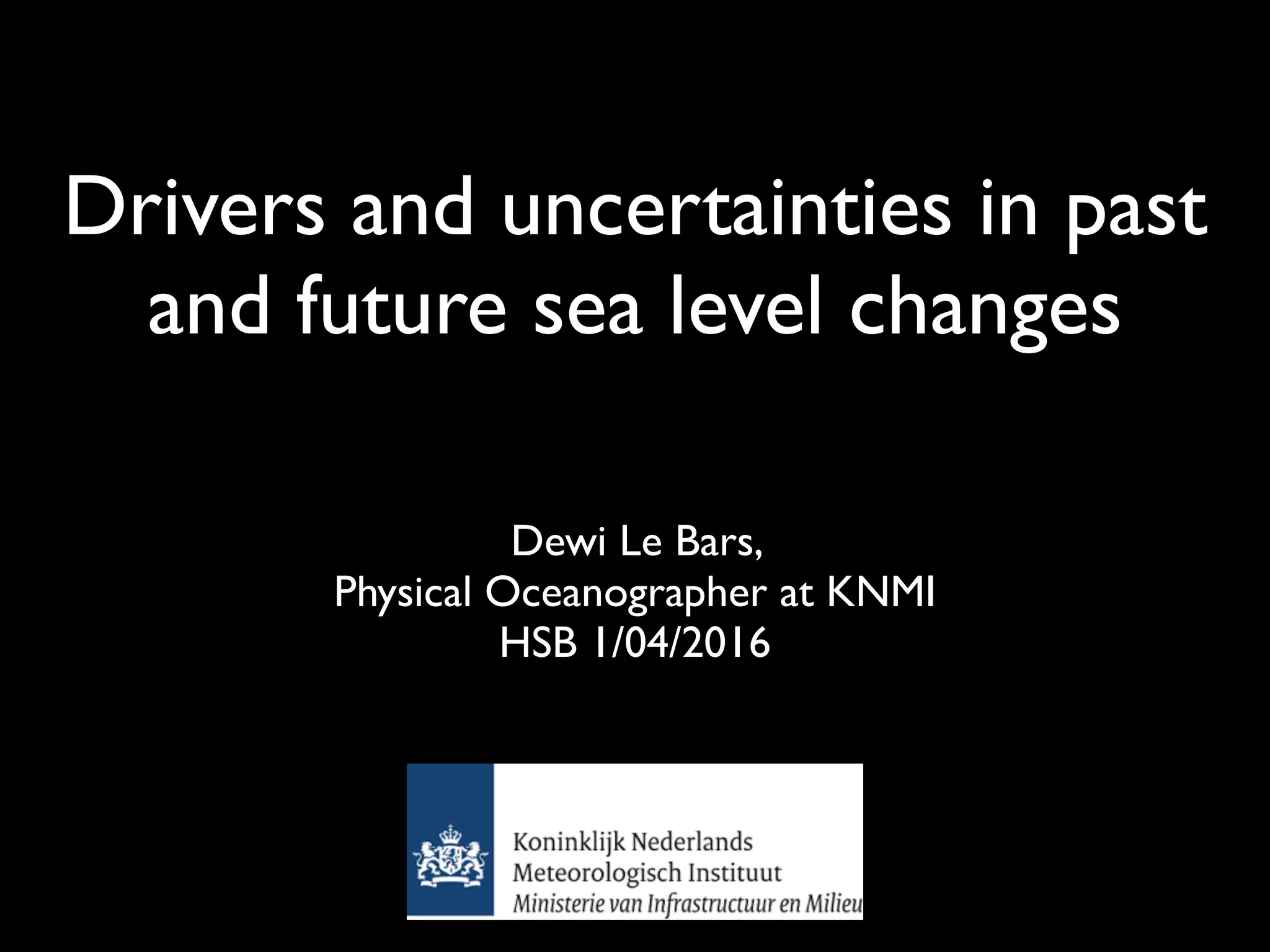
![Past sea level variationsTable 13.1 | Global mean sea level budget (mm yr–1
) over different time intervals from observations and from model-bas
sphere–Ocean General Circulation Model (AOGCM) historical integrations end in 2005; projections for RCP4.5 are used
glacier contributions are computed from the CMIP5 results, using the model of Marzeion et al. (2012a) for glaciers.The land
only, not including climate-related fluctuations.
Source 1901–1990
Observed contributions to global mean sea level (GMSL) rise
Thermal expansion –
Glaciers except in Greenland and Antarcticaa
0.54 [0.47 to 0.61] 0
Glaciers in Greenlanda
0.15 [0.10 to 0.19] 0
Greenland ice sheet –
Antarctic ice sheet –
Land water storage –0.11 [–0.16 to –0.06] 0
Total of contributions –
Observed GMSL rise 1.5 [1.3 to 1.7]
Modelled contributions to GMSL rise
Thermal expansion 0.37 [0.06 to 0.67] 0
Glaciers except in Greenland and Antarctica 0.63 [0.37 to 0.89] 0
Glaciers in Greenland 0.07 [–0.02 to 0.16] 0
Total including land water storage 1.0 [0.5 to 1.4]
Residualc
0.5 [0.1 to 1.0]
different time intervals from observations and from model-based contributions. Uncertainties are 5 to 95%.The Atmo-
ical integrations end in 2005; projections for RCP4.5 are used for 2006–2010. The modelled thermal expansion and
using the model of Marzeion et al. (2012a) for glaciers.The land water contribution is due to anthropogenic intervention
1901–1990 1971–2010 1993–2010
rise
– 0.8 [0.5 to 1.1] 1.1 [0.8 to 1.4]
0.54 [0.47 to 0.61] 0.62 [0.25 to 0.99] 0.76 [0.39 to 1.13]
0.15 [0.10 to 0.19] 0.06 [0.03 to 0.09] 0.10 [0.07 to 0.13]b
– – 0.33 [0.25 to 0.41]
– – 0.27 [0.16 to 0.38]
–0.11 [–0.16 to –0.06] 0.12 [0.03 to 0.22] 0.38 [0.26 to 0.49]
– – 2.8 [2.3 to 3.4]
1.5 [1.3 to 1.7] 2.0 [1.7 to 2.3] 3.2 [2.8 to 3.6]
0.37 [0.06 to 0.67] 0.96 [0.51 to 1.41] 1.49 [0.97 to 2.02]
0.63 [0.37 to 0.89] 0.62 [0.41 to 0.84] 0.78 [0.43 to 1.13]
0.07 [–0.02 to 0.16] 0.10 [0.05 to 0.15] 0.14 [0.06 to 0.23]
1.0 [0.5 to 1.4] 1.8 [1.3 to 2.3] 2.8 [2.1 to 3.5]
0.5 [0.1 to 1.0] 0.2 [–0.4 to 0.8] 0.4 [–0.4 to 1.2]
Last two decades: first closure of the budget (IPCC,AR5)](https://image.slidesharecdn.com/sealevelhsb2016-160406114318/85/Drivers-and-uncertainties-in-past-and-future-sea-level-changes-14-320.jpg)
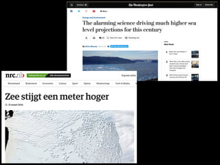
![Future sea level rise
–2013) is about 3.7 mm yr–1
, slightly above the observational
of 3.2 [2.8 to 3.6] mm yr–1
for 1993–2010, because the modelled
butions for recent years, although consistent with observations
93–2010 (Section 13.3), are all in the upper part of the observa-
A1B RCP2.6 RCP4.5 RCP6.0 RCP8.5
0.0
0.2
0.4
0.6
0.8
1.0
1.2
Globalmeansealevelrise(m)
2081-2100 relative to 1986-2005Sum
Thermal expansion
Glaciers
Greenland ice sheet (including dynamics)
Antarctic ice sheet (including dynamics)
Land water storage
Greenland ice-sheet rapid dynamics
Antarctic ice-sheet rapid dynamics
13.10 | Projections from process-based models with likely ranges and median values for global mean sea level rise and its contributions in 2081–2100 relative t
r the four RCP scenarios and scenario SRES A1B used in the AR4.The contributions from ice sheets include the contributions from ice-sheet rapid dynamical chang
due to increasing extraction of groundwater.
(From IPCC,AR5)](https://image.slidesharecdn.com/sealevelhsb2016-160406114318/85/Drivers-and-uncertainties-in-past-and-future-sea-level-changes-16-320.jpg)
![Questions?
References:
Church, J.A., P.U. Clark, A. Cazenave, J.M. Gregory, S. Jevrejeva, A. Levermann, M.A.
Merrifield, G.A. Milne, R.S. Nerem, P.D. Nunn, A.J. Payne, W.T. Pfeffer, D. Stammer and
A.S. Unnikrishnan, 2013: Sea Level Change. In: Climate Change 2013: The Physical Science
Basis. Contribution of Working Group I to the Fifth Assessment Report of the
Intergovernmental Panel on Climate Change [Stocker, T.F., D. Qin, G.-K. Plattner, M.
Tignor, S.K. Allen, J. Boschung, A. Nauels, Y. Xia, V. Bex and P.M. Midgley (eds.)].
Cambridge University Press, Cambridge, United Kingdom and New York, NY, USA
Kopp, R. E., Kemp, A. C., Bittermann, K., Horton, B. P., Donnelly, J. P., Gehrels, W. R., …
Rahmstorf, S. (2016). Temperature-driven global sea-level variability in the Common Era, 1–
8. http://doi.org/10.1073/pnas.1517056113
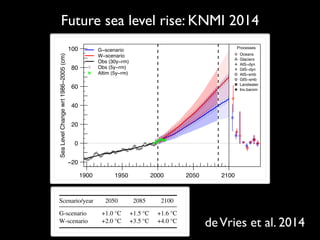
Vries, H. De, Katsman, C., & Drijfhout, S. (2014). Constructing scenarios of regional sea
level change using global temperature pathways. Environmental Research Letters, 9(11),
115007. http://doi.org/10.1088/1748-9326/9/11/115007](https://image.slidesharecdn.com/sealevelhsb2016-160406114318/85/Drivers-and-uncertainties-in-past-and-future-sea-level-changes-20-320.jpg)

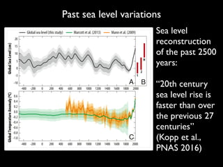
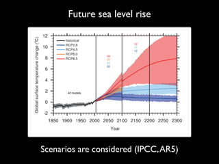
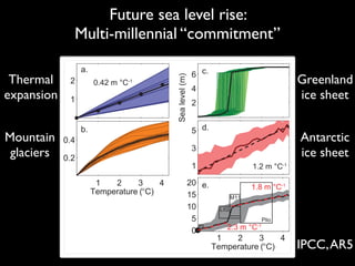
1. Sea level rise is driven by thermal expansion of oceans, melting of land ice such as glaciers and ice sheets, and changes to land water storage. 2. Past rates of sea level rise have varied over time, with the 20th century rise likely the fastest in the past 2700 years. 3. Future projections estimate a rise between 0.5 to over 1 meter by 2100 depending on emissions scenario, with a long term commitment of 1-3 meters of rise for sustained warming over millennia.


![[CM2015] Chapter 9 - Land Ice Modeling](https://cdn.slidesharecdn.com/ss_thumbnails/cm2015-ch09-landice-160120145726-thumbnail.jpg?width=640&height=640&fit=bounds)


