Downloaded 44 times
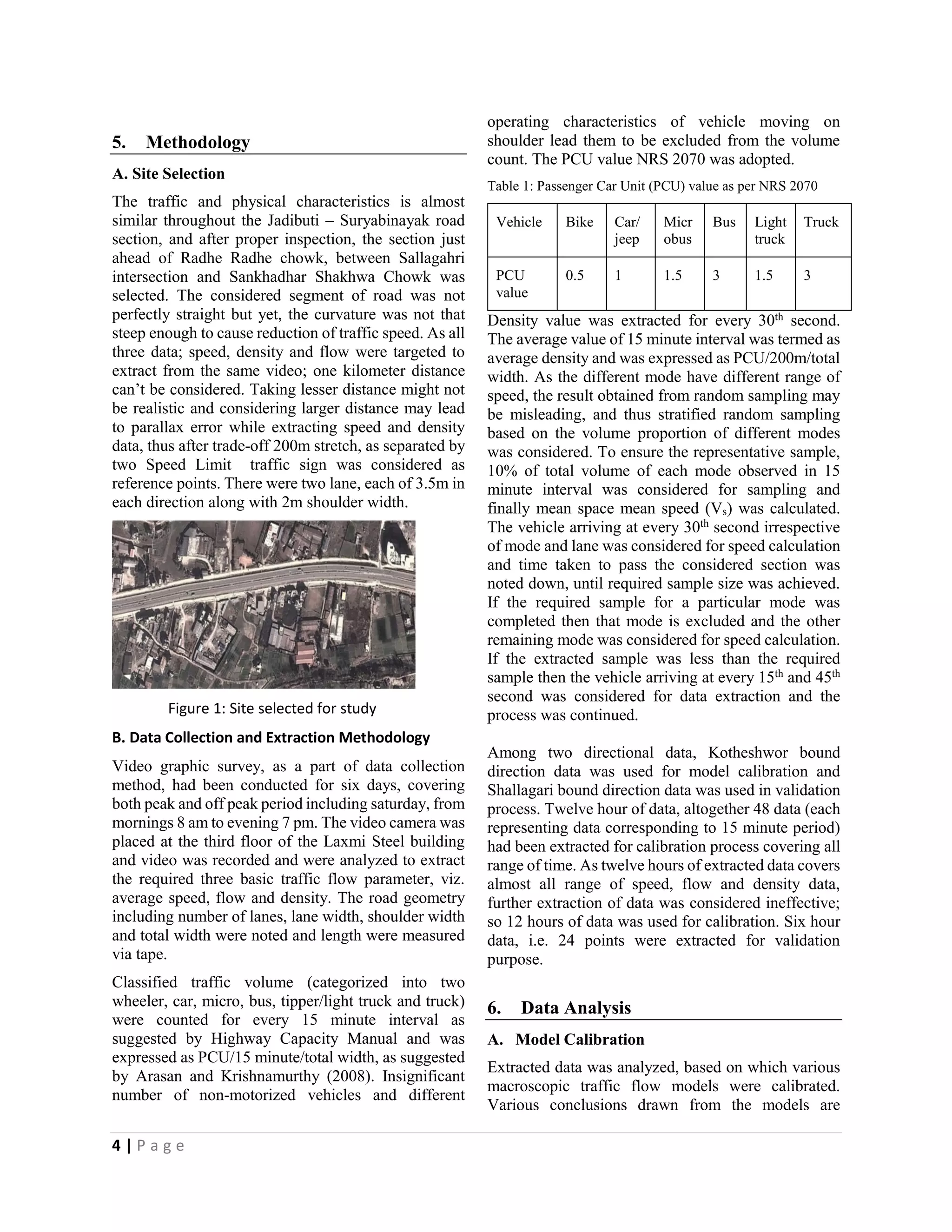
![model shows strong goodness of fit under congested conditions but does not satisfy the boundary condition at low density regime i.e. fails to predict free flow speed.
Underwood’s Exponential Model
Underwood (1961) proposed another exponential form of macroscopic traffic flow model, so as to overcome the drawback of Greenshield model. The Underwood model is expressed mathematically as:
푉=푉푓×푒(−퐾 퐾0⁄) Where, V represents speed corresponding to density K, Vf and Ko represent free flow speed and optimum density (density corresponding to the maximum flow). This model gives better fit than the Greenshields and Greenberg models for the uncongested traffic conditions, but fails to do so for congested conditions. It doesn’t satisfy the boundary condition at high density regime.
Underwood Model with Taylor Series Expansion
Exponential function of Underwood model can be expanded in a Taylor series for the numerical approximation of jam density, which can’t be obtained from conventional Underwood model u= ufe−kkc⁄ = uf(1− kkc+ k22kc2− k36kc3+ k424kc4− k5120kc5+⋯)
Considering up to third degree of k yields u=ufe−kkc⁄ = uf (1− kkc+ k22kc2− k36kc3)
The above equation gives the realistic estimate for the jam density (kj) by substituting u = 0
Drake Model (Bell-Shaped Curve Model)
Drake (1961) improved Underwood model, by proposing bell shaped model after analyzing all model from statistical point of view. He estimate density from speed and flow data, fitted the speed vs. density function and transformed the speed vs. density function to a speed vs. flow function to validate his model. The mathematical expression is:
V=푉푓exp[− 퐾22∗퐾푐 2]
Where, V represents speed corresponding to density k, Kc and Vf represents density corresponding to maximum flow and free flow speed respectively. Drake model generally yields a best fit than other models for uncongested conditions, but fails to provide a good fit for congested conditions.
Pipes-Munjal model Pipes proposed a model with introduction of new parameter (n) to provide a more generalized modeling approach shown by the following equation. When n =1, Pipe's model resembles Greenshields' model. Thus by varying the values of ‘n’, a family of models can be developed.
U= Uf∗{1−( KKj)n}
Where symbol have their usual meanings Polynomial Model: Polynomial models of order 2,3,4 and onwards are calibrated based on the data and are checked for their goodness of fit and other estimate. Density and speed relationship expressed as quadratically (polynomial of order 2) is expressed as:
u = uf+ b*k + c*k2
Where, b and c are additional model parameters, to be determined.
Modified Greenberg Model
Ardekani and Ghandehari (2008) proposed a Modified Greenberg model introducing a non-zero average minimum density, Ko, assuming that there is always some vehicles on the freeway. u=uc∗ln ( kj+kok+ko)
Where Uc and Ko represents speed corresponding to maximum flow and Average minimum density respectively. This model yields a finite free flow speed of Uf=Uc* ln(1 + kj/ko) when density approaches zero. Density at capacity of this model will be kc≈ 0.4kj, a value close to that of the classical Greenberg model, (kc≈ 0.368kj) obtained by solving for dq/dk= 0.
The Drake Model with Taylor Series Expansion
Conventional Drake model can be expanded using Taylor series expansion to obtain a numerical approximation for the jam density, as follows:
u=uf(1− k22kc2+ k48kc4− k648kc6)](https://image.slidesharecdn.com/yiynjf79qdyd8bf59foy-signature-a6015f0ecfba83bfe0d6922aa77b0f8eb53ae8382a0a45291e734842d7763643-poli-140907065955-phpapp01/75/Macroscopic-Traffic-Flow-model-for-nepalese-roads-3-2048.jpg)
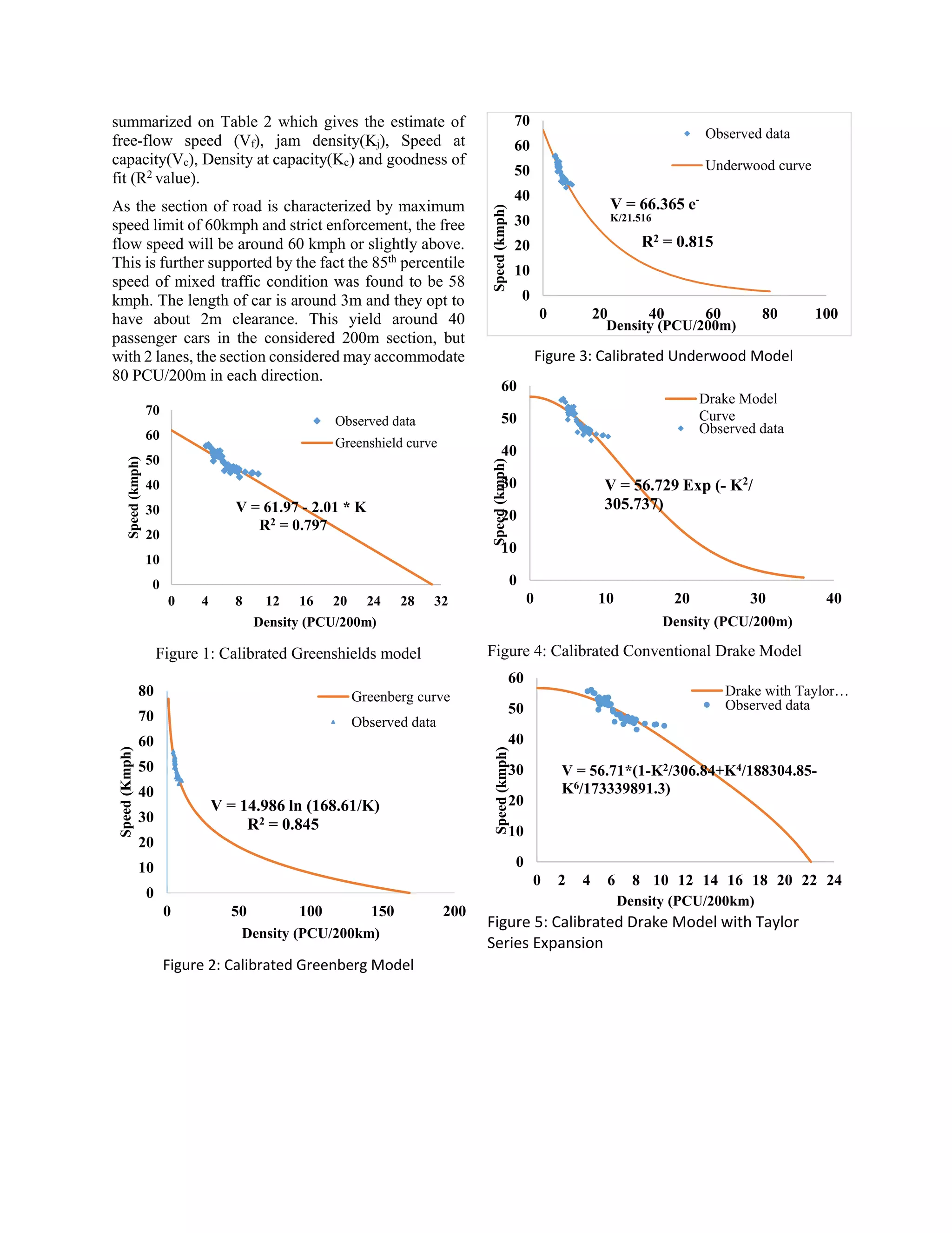
![6 | P a g e
Figure 6: Calibrated Two degree polynomial model
Figure 7: Calibrated Pipes – Munjal Model for N = 2.
Figure 8: Calibrated Underwood Model with Taylor Series Expansion
Table 2: Calibration of various macroscopic traffic flow model
Model
Calibrated Equation
Vf
(kmph)
Vc
(kmph)
Kj
(PCU/200m)
Kc
(PCU/200m)
R2
Greenshields
V = 61.97 (1 – K/30.83)
61.97
30.98
30.83
15.42
0.80
Greenberg
V = 14.99 Ln (168.61/K)
-
14.99
168.61
62.03
0.84
Conventional Underwood
V = 66.36Exp ( -K/21.52)
66.36
24.4 2
-
21.52
0.82
Underwood with Taylor Expansion
V = 66.16 * (1- K/21.8+K2/948.6- K3/61976.96)
66.16
22.05
34.81
21.8
0.82
Conventional Drake
V = 56.73Exp (- K2 / 305.737)
56.73
34.41
-
12.36
0.75
Drake with Taylor Series Expansion
V = 56.71*(1- K2/306.84+K4/188304.85 - K6/173339891.3)
56.71
34.26
22.13
12.39
0.75
Pipes-Munjal(N=2)
U = 55.83 * {1 – (K/19.29)2}
55.83
37.22
19.29
11.14
0.72
Polynomial (N = 2)
V = 0.4018*K2 - 7.7448*K + 81.696
81.69
-
-
-
0.88
0
10
20
30
40
50
60
70
80
90
0
2
4
6
8
10
12
14
Speed (kmph)
Density (PCU/200m)
Two degreepolynomial fit
Observed Data
V = 0.4018*K2-7.7448*K + 81.696R² = 0.8778
0
10
20
30
40
50
60
0
2
4
6
8
10
12
14
16
18
20
22
Speed (Kmph)
Density (PCU/200m)
Pipes-Munjal model (N=2)
Observed Data
V= 55.834*[1- (K/19.29)2]
0
10
20
30
40
50
60
70
0
10
20
30
40
Speed (kmph)
Density (PCU/200m)
Underwood with TaylorExpansion
Observed points
V = 66.16*(1-K/21.8+K2/948.6- K3/61976.96
R2value = 0.814](https://image.slidesharecdn.com/yiynjf79qdyd8bf59foy-signature-a6015f0ecfba83bfe0d6922aa77b0f8eb53ae8382a0a45291e734842d7763643-poli-140907065955-phpapp01/75/Macroscopic-Traffic-Flow-model-for-nepalese-roads-6-2048.jpg)
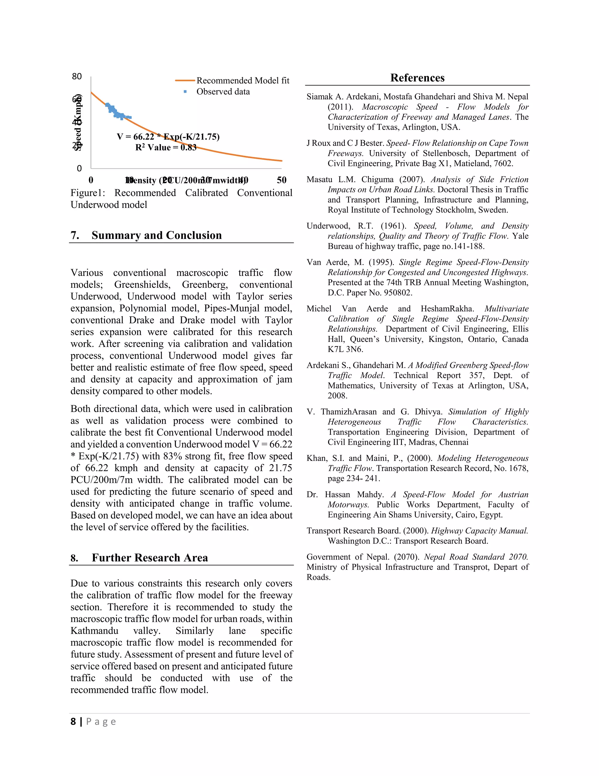

This research focuses on calibrating conventional macroscopic traffic flow models for the Jadibuti-Suryabinayak road section in Nepal, emphasizing the relationship between speed, flow, and density. Various models, including Greenshields, Greenberg, and Underwood, were calibrated and validated, with the Underwood model recommended as the best fit based on its performance metrics. The findings aim to enhance traffic prediction and congestion quantification in the region.