Downloaded 400 times
![Encoder networks
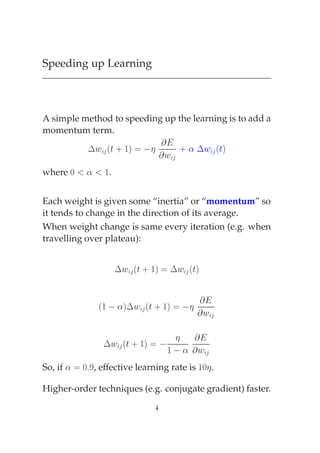
Momentum = 0.9 Learning Rate = 0.25
Error
10.0
0.0
0 402
Input Set[3] Output Set[0]
Pat 1 Pat 1
Pat 2 Pat 2
Pat 3 Pat 3
Pat 4 Pat 4
Pat 5 Pat 5
Pat 6 Pat 6
Pat 7 Pat 7
Pat 8 Pat 8
8 inputs: local encoding, 1 of 8 active.
Task: reproduce input at output layer (“bottleneck”)
After 400 epochs, activation of hidden units:
Pattern Hidden units Pattern Hidden units
1 1 1 1 5 1 0 0
2 0 0 0 6 0 0 1
3 1 1 0 7 0 1 0
4 1 0 1 8 0 1 1
Also called “self-supervised” networks.
Related to PCA (a statistical method).
Application: compression.
Local vs distributed representations.
5](https://image.slidesharecdn.com/bp2slides-090922011749-phpapp02/85/The-Back-Propagation-Learning-Algorithm-5-320.jpg)

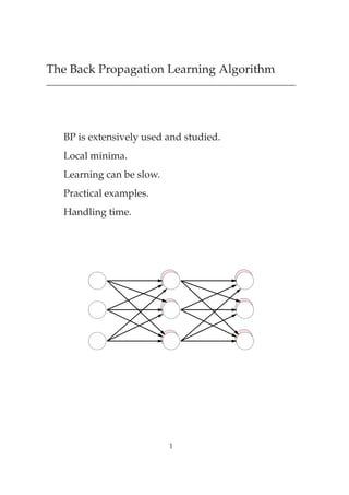
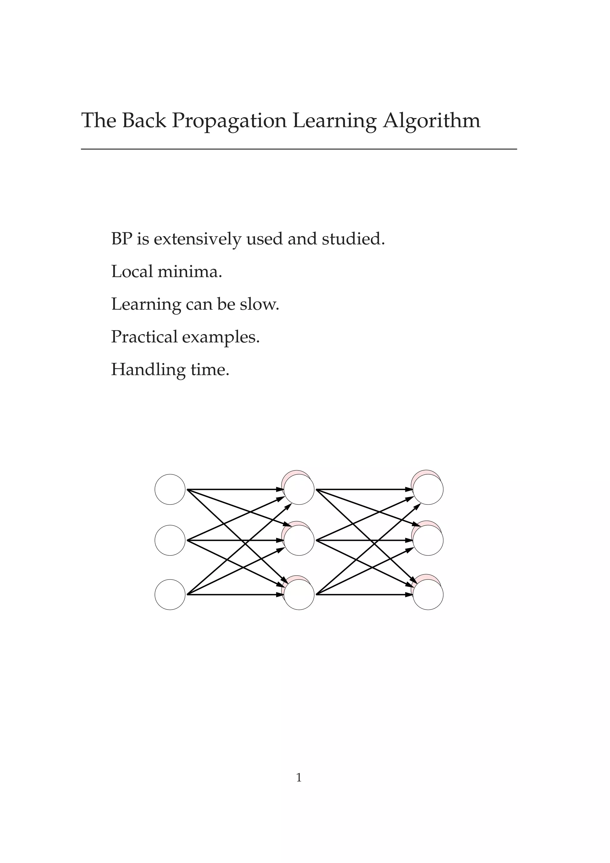
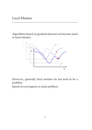
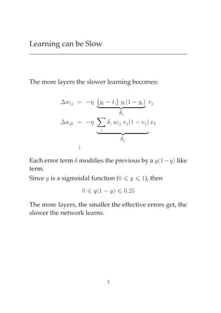
The document discusses the back propagation learning algorithm. It can be slow to train networks with many layers as error signals get smaller with each layer. Momentum and higher-order techniques can speed up learning. Examples are given of applying back propagation to tasks like speech recognition, encoding/decoding patterns, and handwritten digit recognition. While popular, back propagation has limitations like potential local minima issues and lack of biological plausibility in its error backpropagation process.


![[Harvard CS264] 09 - Machine Learning on Big Data: Lessons Learned from Googl...](https://cdn.slidesharecdn.com/ss_thumbnails/machinelearningbigdata-maxlin-cs264opt-110331195757-phpapp01-thumbnail.jpg?width=640&height=640&fit=bounds)


![[DSC 2016] 系列活動:李宏毅 / 一天搞懂深度學習](https://cdn.slidesharecdn.com/ss_thumbnails/1-160521014039-thumbnail.jpg?width=640&height=640&fit=bounds)


