The document provides an overview of machine learning, focusing on artificial neural networks (ANN) and the perceptron algorithm for supervised learning. It explains various machine learning approaches, the structure of ANNs, the perceptron learning process, and principles such as bias and learning rate. Additionally, it includes a simple perceptron example and homework assignments related to designing an ANN and applying the perceptron algorithm.

1. Perceptron in ANN
UNIVERSITY OF BABYLON
IT FACULTY
SOFTWARE DEPARTMENT
MODULE: ARTIFICIAL INTELLIGENCE
STAGE: 3
ZAID A. AL-HUSSEINI
2018-2019

2. Introduction: What is Machine
Learning?
 Machine Learning (ML): is the scientific of algorithms and
statistical models that computer systems use to perform a
specific task without using explicit instructions.
 It rely on patterns and inference instead.
2

3. Introduction: What is Machine
Learning?
 Machine Learning is widely used in email filtering, computer
vision, recommendation engines, Insurance, and many other
fields.
 Machine Learning algorithms build a mathematical model
based on sample data, known as "training dataset”.
3

4. Machine Learning approaches
 1. Supervised Machine Learning: build a mathematical model
by using data that contains both the inputs and the desired
outputs. The data is known as training data, and consists of a
set of training examples.
 2. Unsupervised Machine Learning: take a set of data that
contains only inputs, and find structure in the data, like
grouping or clustering of data points.
4

5. Machine Learning approaches
 3. Reinforcement Machine Learning: A process of trial and
error designed to maximize the expected value of a criterion
function. If an action is followed by an improved “state”, the
action should be strengthened, and vice versa.
5

6. Artificial Neural Networks (ANN)
 Artificial neural networks (ANN) are computing systems
inspired by the biological neural networks .
 Such systems "learn" to perform tasks by considering
examples.
 An ANN is based on a collection of connected units or nodes
called artificial neurons. These nodes are connected to each
other by “edges”. These connections have a “weight”.
6

7. Artificial Neural Networks (ANN) 7

8. Artificial Neural Networks (ANN)
 Artificial neural networks (ANN) are composed of three
layers:
1. Input layer.
2. Output layer.
3. Hidden layer.
 By moving the data through these layers, the network will
adjust its weights as a result of the learning process.
8

9. Perceptron
 The perceptron is an algorithm for supervised learning of
binary linear classifiers.
 The perceptron can be seen as
the simplest kind of feed
forward neural network.
 The idea behind it is to consider
every pattern in the input data
and compare the result to the
real output, and adjust the
weights.
9

10. Perceptron learning process
1. Get the labelled training dataset (array of input(s) and output(s)).
2. Initial the weight(s) into random values.
3. Calculate the sum of the perceptron by using the equation:
𝒔𝒖𝒎 =
𝒊=𝟎
𝜼
𝒘𝒊 ∗ 𝒙𝒊
10

11. Perceptron learning process
4. Apply activation function on the sum function to calculate the Actual
Output by using the equation of Hard Limits:
𝒐𝒖𝒕𝒑𝒖𝒕 =
𝟏 𝒊𝒇 𝒔𝒖𝒎 > 𝟎
−𝟏 𝒐𝒕𝒉𝒆𝒓𝒘𝒊𝒔𝒆
Note that there are many other methods to apply the activation function.
11

12. Perceptron learning process
5. Calculate the Local Error (desired output – actual output) by using the
equation:
𝑳𝒐𝒄𝒂𝒍 𝑬𝒓𝒓𝒐𝒓 = 𝒀 − 𝒐𝒖𝒕𝒑𝒖𝒕
6. Calculate the Global Error by summing the absolute value of the local
error.
12

13. Perceptron learning process
7. If the local error is not zero, update the weight by using the equation:
𝜟𝑾𝒊𝒋 = 𝑳𝒆𝒂𝒓𝒏𝒊𝒏𝒈 𝑹𝒂𝒕𝒆 ∗ 𝑳𝒐𝒄𝒂𝒍 𝑬𝒓𝒓𝒐𝒓𝒊 ∗ 𝑰𝒏𝒑𝒖𝒕𝒊
8. Repeat the previous steps (iterations) until the Global Error is zero. And
calculate the number of iterations until we get the minimum error.
13

14. Perceptron learning example
 Let assume we want a simple perceptron to be trained on logical AND
gate operator. So the training dataset will be:
X1 X2 Y
0 0 0
0 1 1
1 0 1
1 1 1
 Assume the threshold value is 0.2.
 Assume the learning rate is 0.1.
14

15. Perceptron learning example 15

16. Algorithm of Perceptron
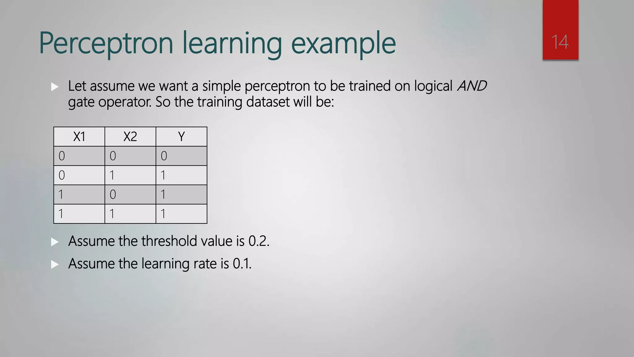
 Get the training data (inputs and outputs).
 Set the weights (W1 and W2) to random values.
 While Global Error is not zero
 For each input value in the training dataset
 Calculate the output of the perceptron. By
1. Sum = Input1[i] * W1 + Input2[i] * W2
2. Apply activation function (e.g. Hard Limits)
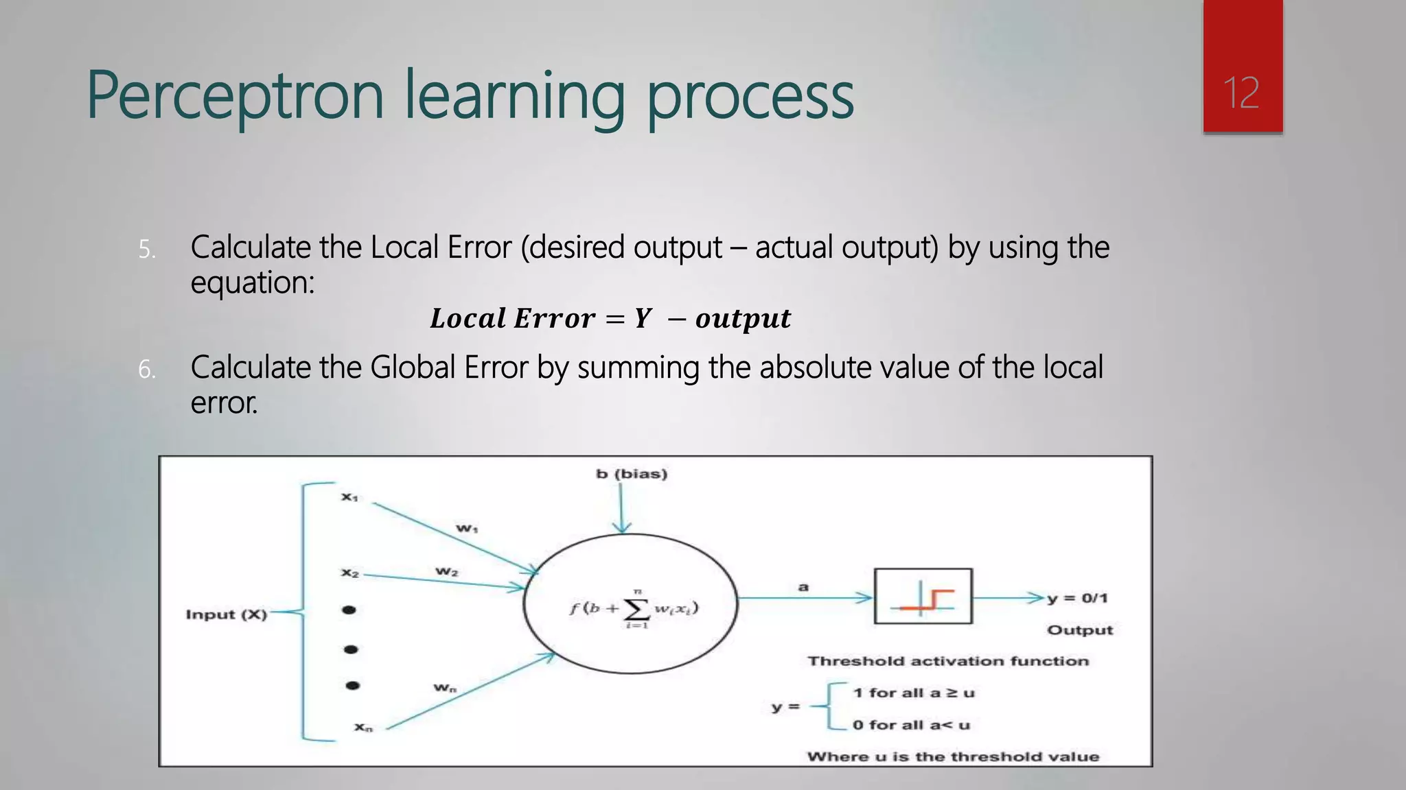
 Calculate the Local Error for this input. By
Local Error = Desired output – Actual output
 If the Local Error is not zero, update both weights (W1 and W2) by
W[ j]=w[ j] + Learning rate * Local Error * Input[i][ j]
 Global Error += Absolute of Local Error
 End for
 End while
16

17. Some principles we used
 Bias: The Bias is used when calculating the input value of a
neuron, in this equation:
output = sum (weights * inputs) + bias
 Usually the Bias value is 1. And by adjusting its weight, it allow us to
modify the direction and derivate of the model classifier.
 Learning Rate: determine the learning speed to find the
optimal solution. If the Learning Rate value is low, it will find a
better solution, but it will be computationally cost. And if the
value is high, it will be fast in finding a solution, but this
solution is not necessarily the best solution.
17

18. Some principles we used
 Iteration: is the number of loops on the training dataset to
find the optimal values of the weights (reach to the expected
global error). We should have one iteration at least.
 Local and Global Error: Local Error is the difference between
the calculated output of the training inputs, and the desired
output in the training dataset. While global error is the
summation of the absolute values of the local error for each
pattern in a single iteration.
18

19. Homework
 H.W 1: Design an ANN for a problem of your choice.
 H.W 2: Apply the algorithm in Java or C#, with OR training
dataset.
 H.W 3: Plot the data and the generated model on 2-dimentions
graph.
 H.W 4: Use the generated model to predict the new data.
19