HOPFIELD NETWORK

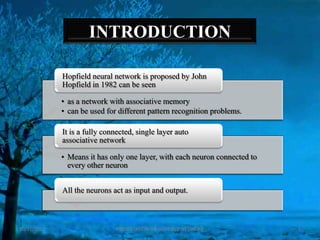
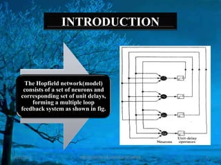
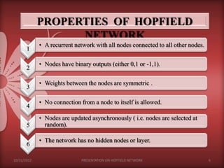
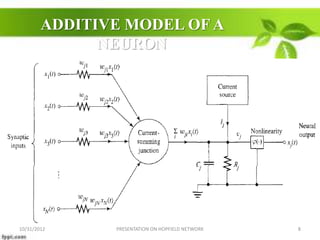
PRESENTED BY :
Ankita Pandey
ME ECE - 112604

CONTENT
Introduction

Properties of Hopfield network

Hopfield network derivation

Hopfield network example

Applications

References

10/31/2012 PRESENTATION ON HOPFIELD NETWORK 2

INTRODUCTION

Hopfield neural network is proposed by John
Hopfield in 1982 can be seen

• as a network with associative memory
• can be used for different pattern recognition problems.

It is a fully connected, single layer auto
associative network

• Means it has only one layer, with each neuron connected to
every other neuron

All the neurons act as input and output.


INTRODUCTION

The Hopfield network(model)
consists of a set of neurons and
corresponding set of unit delays,
forming a multiple loop
feedback system as shown in fig.


INTRODUCTION

The number of feedback loops is equal to
the number of neurons.

Basically, the output of the neuron is
feedback, via a unit delay element, to
each of the other neurons in the network.

• no self feedback in the network.


PROPERTIES OF HOPFIELD
NETWORK
• A recurrent network with all nodes connected to all other nodes.
1

• Nodes have binary outputs (either 0,1 or -1,1).
2

• Weights between the nodes are symmetric .
3

• No connection from a node to itself is allowed.
4
• Nodes are updated asynchronously ( i.e. nodes are selected at
5 random).

• The network has no hidden nodes or layer.
6


HOPFIELD NETWORK
Consider the noiseless, dynamical model of the neuron shown
in fig. 1

The synaptic weights w j1
,w j2
,...... w jn represents
conductance’s.

The respective inputs x1 t , x 2 t ,...... x n t represents
the potentials, N is number of inputs.

These inputs are applied to a current summing junction
characterized as follows:
• Low input resistance.
• Unity current gain.
• High output resistance.


ADDITIVE MODEL OF A
NEURON
di

ei

Σ
NEURAL
NETWORK
MODEL yi


HOPFIELD NETWORK
The total current flowing toward the input node of the nonlinear
element(activation function) is:
N

w ji
xi t Ii
i 1

Total current flowing away from the input node of the nonlinear
element as follows:
v j
t dv j
t
C j
R j
dt
• Where first term due to leakage resistance
• And second term due to leakage capacitance.


HOPFIELD NETWORK
• By applying KCL to the input node of the nonlinearity , we
get
N
dv j t vj t
Cj w ji x i t Ij
dt Rj i 1
………..(1)
dv t
• The capacitive term C dt
j
j
add dynamics to the model
of a neuron.
• Output of the neuron j determined by using the non linear
relation
xj t v j (t )
• The RC model described by the eq. (1) is referred to the
additive model


HOPFIELD NETWORK
A feature of Additive model is that the signal xᵢ(t) applied to the
neuron j by adjoining neuron i

• is a slowly varying function of the time t.

Thus, a recurrent network consisting of an interconnection of N
neurons,

• each one of which is assumed to have the same mathematical
model described by thev j t
dv j t equation : N
Cj w ji x i t I j,
dt Rj i 1

• j 1, 2 ,....., N
• …….(2)

HOPFIELD NETWORK
Now, we use eq (2) which is based on the additive model of the
neuron.

Assumptions:

w ji w ij
• The matrix of synaptic weights is symmetric, as shown by:
• for all i and j.
• Each neuron has a nonlinear activation of its own, hence use
of i in eq.(2)
• The inverse of the nonlinear activation function exists, so we
can write
1
• v i
x
……….(3)

HOPFIELD
NETWORK hyperbolic tangent
• Let the sigmoid function v
be defined by the
i

function
aiv 1 exp aiv
x i
v tanh
2 1 exp aiv
• Which has slope of a i / 2.
• a i refers as the gain of neuron i.
The inverse I/O relation of eq.(3) may be written as
1 1 1 x
v x log
ai 1 x
………..(4)


HOPFIELD
•
NETWORK
Standard form of the inverse I/O relation for a neuron of unity gain is:
1 1 x
x log
1 x
• We can rewrite the eq. (4) in terms of standard relation as
1 1 1
i
x x
ai


Plot of (a) Sigmoidal Nonlinearity and (b) its
inverse

Error
ei

Model
UNKNOW Output xi
N
SYSTEM Σ
f(.)

(a) (b)
10/31/2012
yi PRESENTATION ON HOPFIELD NETWORK 15

HOPFIELD
NETWORK
• The energy function of the Hopfield network is defined by:
x j
N N N N
1 1 1
E w ji
xi x j j
x dx I jx j
2 i 1 j 1 j 1 R j 0 j 1

• Differentiating E w.r.t. time , we get
N N
dE v j
dx j
w ji
xi I j
dt j 1 i 1 R j
dt

• by putting the value in parentheses from eq.2, we get
N
dE dv j
dx j

dt
C j
dt dt
…………..(5)
j 1


HOPFIELD
• The inverse relation NETWORK is
that defines in terms of x v j j
1
v i
x
• By using above relation in eq. (5), we have
N 1
dE d j
x j
dx j
C j
dt j 1 dt dt
2 1
N
dx j
d j
x j
C j
dt dx …………..(6)
j 1 j

• From fig. (b) we see that the inverse I/O relation is monotonically
increasing function of the output
Therefore,


HOPFIELD
Also,
NETWORK 2
dx j
0 for all x j .
dt
Hence all the factors that make up the sum on R.H.S. of eq(6) are non-
negative.
Thus the energy function E defined as
dE
0
dt


HOPFIELD
NETWORK
• The energy function E is a Lyapunov
funtion of the continuous Hopfield model.
We may make the • The model is stable in accordance with
following two Lyapunov’s Theorem 1.
statements:

The time evolution of the • Which seeks the minima of the energy
continuous Hopfield model function E and comes to stop at fixed
described by the system of points.
nonlinear first order
differential equations
represents the trajectory in
the state space


HOPFIELD
NETWORK dE
• From eq.(6) the derivative vanishes only if
dt

dx j
t
0 for all j.
dt
• Thus we can say,
dE
0 expect at fixed point ………(7)
dt

• The eq.(7) forms the basis for following theorem
• The energy function E of a Hopfield network is a monotonically
decreasing function of time.


HOPFIELD NETWORK
EXAMPLE
Connection of Hopfield Neural Network A Hopfield Neural network:

Neuron Neuron Neuron Neuron
1 (N1) 2 (N2) 3 (N3) 4 (N4)

Neuron
(N/A) N2->N1 N3->N1 N4->N1
1 (N1)

Neuron
N1->N2 (N/A) N3->N2 N4->N2
2 (N2)

Neuron
N1->N3 N2->N3 (N/A) N4->N3
3 (N3)

Neuron
N1->N4 N2->N4 N3->N4 (N/A)
4 (N4)10/31/2012 PRESENTATION ON HOPFIELD NETWORK 21

HOPFIELD NETWORK
EXAMPLE
• The connection weights put into this array, also called a weight matrix, allow
the neural network to recall certain patterns when presented.
• For example, the values shown in Table below show the correct values to use to
recall the patterns 0101 .

Neuron 1 Neuron 2 Neuron 3 Neuron 4
Weight Matrix used
(N1) (N2) (N3) (N4)
to recall 0101.
Neuron 1
0 -1 1 -1
(N1)

Neuron 2
-1 0 -1 1
(N2)

Neuron 3
1 -1 0 -1
(N3)

Neuron 4
-1 1 -1 0
(N4)

Calculating The Weight Matrix

Step 1: Convert 0101 to bipolar

• Bipolar is nothing more than a way to represent binary
values as –1’s and 1’s rather than zero and 1’s.
• To convert 0101 to bipolar we convert all of the zeros to –
1’s. This results in:
• 0 = -1
1=1
0 = -1
1=1
• The final result is the array (-1, 1, -1, 1)


 Step 2: Multiply (-1, 1, -1, 1) by its Inverse

For this step we will consider -1, 1, -1, 1 to be a matrix.

Taking the inverse of this matrix we have.

Now, multiply these two matrices
-1 X (-1) = 1 1 X (-1) = -1 -1 X (-1) = 1 1 X (-1) = -1
-1 X 1 = -1 1X1=1 -1 X 1 = -1 1X1=1
-1 X (-1) = 1 1 X (-1) = -1 -1 X (-1) = 1 1 X (-1) = -1
-1 X 1 = -1 1X1=1 -1 X 1 = -1 1X1=1

• And the matrix is:

 Step 3: Set the Northwest diagonal to zero

• The reason behind this is, in Hopfield networks do not have their neurons
connected to themselves.
• So positions [1][1], [2][2], [3][3] and [4][4] in our two dimensional array
or matrix, get set to zero. This results in the weight matrix for the bit pattern
0101.

Recalling Pattern
• To do this we present each input neuron, with the pattern. Each neuron will
activate based upon the input pattern.
• For example, when neuron 1 is presented with 0101 its activation will be the
sum of all weights that have a 1 in input pattern.
• The activation of each neuron is:
a b c d a+b+c+
d
N1 0 -1 0 -1 -2
N2 0 1 0 0 1
N3 0 -1 0 -1 -2
N4 0 1 0 0 1
The final output vector then (-2,1,-2,1)

Recalling Pattern
Now, Threshold value determines what range of values will cause the
neuron to fire.

The threshold usually used for a Hopfield network, is any value greater
than zero.

So the following neurons would fire.

N1 activation is –2, would not fire (0)
N2 activation is 1, would fire (1)
N3 activation is –2, would not fire(0)
N4 activation is 1 would fire (1).


Recalling Pattern

We assign a binary 1 to all neurons that fired, and a binary 0 to all
neurons that do not fire.

The final binary output from the Hopfield network would be 0101.

This is the same as the input pattern.

An auto associative neural network, such as a Hopfield network

Will echo a pattern back if the pattern is recognized.

APPLICATION

Image Detection and Recognition

Enhancing X-Ray Images

In Medical Image Restoration


References

• Jacek M. Zurada, Introduction To Artificial Neural Systems (10th
edition)
• Simon Haykin, Neural Networks (2nd edition)
• Satish Kumar, Neural Networks; A Classroom Approach (2nd
Edition)
• http://www.learnartificialneuralnetworks.com/hopfield.html
• http://www.heatonresearch.com/articles/2/page6.html
• http://www.thebigblob.com/hopfield-network/#associative-memory
•http://www.dsi.unive.it/~pelillo/Didattica/RetiNeurali/Introduction_To
_ANN_lesson_6.pdf.
• http://en.wikipedia.org/wiki/Hopfield_network.


HOPFIELD NETWORK

More Related Content

What's hot

Similar to HOPFIELD NETWORK

Recently uploaded

HOPFIELD NETWORK