This document discusses various importance sampling methods for approximating Bayes factors, which are used for Bayesian model selection. It compares regular importance sampling, bridge sampling, harmonic means, mixtures to bridge sampling, and Chib's solution. An example application to probit modeling of diabetes in Pima Indian women is presented to illustrate regular importance sampling. Markov chain Monte Carlo methods like the Metropolis-Hastings algorithm and Gibbs sampling can be used to sample from the probit models.

1. On approximating Bayes factors
On approximating Bayes factors
Christian P. Robert
Universit´ Paris Dauphine & CREST-INSEE
e
http://www.ceremade.dauphine.fr/~xian
CRiSM workshop on model uncertainty
U. Warwick, May 30, 2010
Joint works with N. Chopin, J.-M. Marin, K. Mengersen
& D. Wraith

2. On approximating Bayes factors
Outline
1 Introduction
2 Importance sampling solutions compared
3 Nested sampling

3. On approximating Bayes factors
Introduction
Model choice
Model choice as model comparison
Choice between models
Several models available for the same observation
Mi : x ∼ fi (x|θi ), i∈I
where I can be finite or infinite
Replace hypotheses with models

4. On approximating Bayes factors
Introduction
Model choice
Model choice as model comparison
Choice between models
Several models available for the same observation
Mi : x ∼ fi (x|θi ), i∈I
where I can be finite or infinite
Replace hypotheses with models

5. On approximating Bayes factors
Introduction
Model choice
Bayesian model choice
Probabilise the entire model/parameter space
allocate probabilities pi to all models Mi
define priors πi (θi ) for each parameter space Θi
compute
pi fi (x|θi )πi (θi )dθi
Θi
π(Mi |x) =
pj fj (x|θj )πj (θj )dθj
j Θj
take largest π(Mi |x) to determine “best” model,

6. On approximating Bayes factors
Introduction
Model choice
Bayesian model choice
Probabilise the entire model/parameter space
allocate probabilities pi to all models Mi
define priors πi (θi ) for each parameter space Θi
compute
pi fi (x|θi )πi (θi )dθi
Θi
π(Mi |x) =
pj fj (x|θj )πj (θj )dθj
j Θj
take largest π(Mi |x) to determine “best” model,

7. On approximating Bayes factors
Introduction
Model choice
Bayesian model choice
Probabilise the entire model/parameter space
allocate probabilities pi to all models Mi
define priors πi (θi ) for each parameter space Θi
compute
pi fi (x|θi )πi (θi )dθi
Θi
π(Mi |x) =
pj fj (x|θj )πj (θj )dθj
j Θj
take largest π(Mi |x) to determine “best” model,

8. On approximating Bayes factors
Introduction
Model choice
Bayesian model choice
Probabilise the entire model/parameter space
allocate probabilities pi to all models Mi
define priors πi (θi ) for each parameter space Θi
compute
pi fi (x|θi )πi (θi )dθi
Θi
π(Mi |x) =
pj fj (x|θj )πj (θj )dθj
j Θj
take largest π(Mi |x) to determine “best” model,

9. On approximating Bayes factors
Introduction
Bayes factor
Bayes factor
Definition (Bayes factors)
For comparing model M0 with θ ∈ Θ0 vs. M1 with θ ∈ Θ1 , under
priors π0 (θ) and π1 (θ), central quantity
f0 (x|θ0 )π0 (θ0 )dθ0
π(Θ0 |x) π(Θ0 ) Θ0
B01 = =
π(Θ1 |x) π(Θ1 )
f1 (x|θ)π1 (θ1 )dθ1
Θ1
[Jeffreys, 1939]

10. On approximating Bayes factors
Introduction
Evidence
Evidence
Problems using a similar quantity, the evidence
Zk = πk (θk )Lk (θk ) dθk ,
Θk
aka the marginal likelihood.
[Jeffreys, 1939]

11. On approximating Bayes factors
Importance sampling solutions compared
A comparison of importance sampling solutions
1 Introduction
2 Importance sampling solutions compared
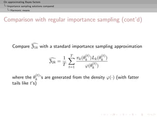
Regular importance
Bridge sampling
Harmonic means
Mixtures to bridge
Chib’s solution
The Savage–Dickey ratio
3 Nested sampling
[Marin & Robert, 2010]

12. On approximating Bayes factors
Importance sampling solutions compared
Regular importance
Bayes factor approximation
When approximating the Bayes factor
f0 (x|θ0 )π0 (θ0 )dθ0
Θ0
B01 =
f1 (x|θ1 )π1 (θ1 )dθ1
Θ1
use of importance functions 0 and 1 and
n−1
0
n0 i i
i=1 f0 (x|θ0 )π0 (θ0 )/
i
0 (θ0 )
B01 =
n−1
1
n1 i i
i=1 f1 (x|θ1 )π1 (θ1 )/
i
1 (θ1 )

13. On approximating Bayes factors
Importance sampling solutions compared
Regular importance
Diabetes in Pima Indian women
Example (R benchmark)
“A population of women who were at least 21 years old, of Pima
Indian heritage and living near Phoenix (AZ), was tested for
diabetes according to WHO criteria. The data were collected by
the US National Institute of Diabetes and Digestive and Kidney
Diseases.”
200 Pima Indian women with observed variables
plasma glucose concentration in oral glucose tolerance test
diastolic blood pressure
diabetes pedigree function
presence/absence of diabetes

14. On approximating Bayes factors
Importance sampling solutions compared
Regular importance
Probit modelling on Pima Indian women
Probability of diabetes function of above variables
P(y = 1|x) = Φ(x1 β1 + x2 β2 + x3 β3 ) ,
Test of H0 : β3 = 0 for 200 observations of Pima.tr based on a
g-prior modelling:
β ∼ N3 (0, n XT X)−1
[Marin & Robert, 2007]

15. On approximating Bayes factors
Importance sampling solutions compared
Regular importance
Probit modelling on Pima Indian women
Probability of diabetes function of above variables
P(y = 1|x) = Φ(x1 β1 + x2 β2 + x3 β3 ) ,
Test of H0 : β3 = 0 for 200 observations of Pima.tr based on a
g-prior modelling:
β ∼ N3 (0, n XT X)−1
[Marin & Robert, 2007]

16. On approximating Bayes factors
Importance sampling solutions compared
Regular importance
MCMC 101 for probit models
Use of either a random walk proposal
β =β+
in a Metropolis-Hastings algorithm (since the likelihood is
available) or of a Gibbs sampler that takes advantage of the
missing/latent variable
z|y, x, β ∼ N (xT β, 1) Iy × I1−y
z≥0 z≤0
(since β|y, X, z is distributed as a standard normal)
[Gibbs three times faster]

17. On approximating Bayes factors
Importance sampling solutions compared
Regular importance
MCMC 101 for probit models
Use of either a random walk proposal
β =β+
in a Metropolis-Hastings algorithm (since the likelihood is
available) or of a Gibbs sampler that takes advantage of the
missing/latent variable
z|y, x, β ∼ N (xT β, 1) Iy × I1−y
z≥0 z≤0
(since β|y, X, z is distributed as a standard normal)
[Gibbs three times faster]

18. On approximating Bayes factors
Importance sampling solutions compared
Regular importance
MCMC 101 for probit models
Use of either a random walk proposal
β =β+
in a Metropolis-Hastings algorithm (since the likelihood is
available) or of a Gibbs sampler that takes advantage of the
missing/latent variable
z|y, x, β ∼ N (xT β, 1) Iy × I1−y
z≥0 z≤0
(since β|y, X, z is distributed as a standard normal)
[Gibbs three times faster]

19. On approximating Bayes factors
Importance sampling solutions compared
Regular importance
Importance sampling for the Pima Indian dataset
Use of the importance function inspired from the MLE estimate
distribution
ˆ ˆ
β ∼ N (β, Σ)
R Importance sampling code
model1=summary(glm(y~-1+X1,family=binomial(link="probit")))
is1=rmvnorm(Niter,mean=model1$coeff[,1],sigma=2*model1$cov.unscaled)
is2=rmvnorm(Niter,mean=model2$coeff[,1],sigma=2*model2$cov.unscaled)
bfis=mean(exp(probitlpost(is1,y,X1)-dmvlnorm(is1,mean=model1$coeff[,1],
sigma=2*model1$cov.unscaled))) / mean(exp(probitlpost(is2,y,X2)-
dmvlnorm(is2,mean=model2$coeff[,1],sigma=2*model2$cov.unscaled)))

20. On approximating Bayes factors
Importance sampling solutions compared
Regular importance
Importance sampling for the Pima Indian dataset
Use of the importance function inspired from the MLE estimate
distribution
ˆ ˆ
β ∼ N (β, Σ)
R Importance sampling code
model1=summary(glm(y~-1+X1,family=binomial(link="probit")))
is1=rmvnorm(Niter,mean=model1$coeff[,1],sigma=2*model1$cov.unscaled)
is2=rmvnorm(Niter,mean=model2$coeff[,1],sigma=2*model2$cov.unscaled)
bfis=mean(exp(probitlpost(is1,y,X1)-dmvlnorm(is1,mean=model1$coeff[,1],
sigma=2*model1$cov.unscaled))) / mean(exp(probitlpost(is2,y,X2)-
dmvlnorm(is2,mean=model2$coeff[,1],sigma=2*model2$cov.unscaled)))

21. On approximating Bayes factors
Importance sampling solutions compared
Regular importance
Diabetes in Pima Indian women
Comparison of the variation of the Bayes factor approximations
based on 100 replicas for 20, 000 simulations from the prior and
the above MLE importance sampler
5
4
q
3
2
Monte Carlo Importance sampling

22. On approximating Bayes factors
Importance sampling solutions compared
Bridge sampling
Bridge sampling
Special case:
If
π1 (θ1 |x) ∝ π1 (θ1 |x)
˜
π2 (θ2 |x) ∝ π2 (θ2 |x)
˜
live on the same space (Θ1 = Θ2 ), then
n
1 π1 (θi |x)
˜
B12 ≈ θi ∼ π2 (θ|x)
n π2 (θi |x)
˜
i=1
[Gelman & Meng, 1998; Chen, Shao & Ibrahim, 2000]

23. On approximating Bayes factors
Importance sampling solutions compared
Bridge sampling
Bridge sampling variance
The bridge sampling estimator does poorly if
2
var(B12 ) 1 π1 (θ) − π2 (θ)
2 ≈ E
B12 n π2 (θ)
is large, i.e. if π1 and π2 have little overlap...

24. On approximating Bayes factors
Importance sampling solutions compared
Bridge sampling
Bridge sampling variance
The bridge sampling estimator does poorly if
2
var(B12 ) 1 π1 (θ) − π2 (θ)
2 ≈ E
B12 n π2 (θ)
is large, i.e. if π1 and π2 have little overlap...

25. On approximating Bayes factors
Importance sampling solutions compared
Bridge sampling
(Further) bridge sampling
General identity:
π2 (θ|x)α(θ)π1 (θ|x)dθ
˜
B12 = ∀ α(·)
π1 (θ|x)α(θ)π2 (θ|x)dθ
˜
n1
1
π2 (θ1i |x)α(θ1i )
˜
n1
i=1
≈ n2 θji ∼ πj (θ|x)
1
π1 (θ2i |x)α(θ2i )
˜
n2
i=1

26. On approximating Bayes factors
Importance sampling solutions compared
Bridge sampling
Optimal bridge sampling
The optimal choice of auxiliary function is
n1 + n2
α =
n1 π1 (θ|x) + n2 π2 (θ|x)
leading to
n1
1 π2 (θ1i |x)
˜
n1 n1 π1 (θ1i |x) + n2 π2 (θ1i |x)
i=1
B12 ≈ n2
1 π1 (θ2i |x)
˜
n2 n1 π1 (θ2i |x) + n2 π2 (θ2i |x)
i=1
Back later!

27. On approximating Bayes factors
Importance sampling solutions compared
Bridge sampling
Optimal bridge sampling (2)
Reason:
Var(B12 ) 1 π1 (θ)π2 (θ)[n1 π1 (θ) + n2 π2 (θ)]α(θ)2 dθ
2 ≈ 2 −1
B12 n1 n2 π1 (θ)π2 (θ)α(θ) dθ
(by the δ method)
Drawback: Dependence on the unknown normalising constants
solved iteratively

28. On approximating Bayes factors
Importance sampling solutions compared
Bridge sampling
Optimal bridge sampling (2)
Reason:
Var(B12 ) 1 π1 (θ)π2 (θ)[n1 π1 (θ) + n2 π2 (θ)]α(θ)2 dθ
2 ≈ 2 −1
B12 n1 n2 π1 (θ)π2 (θ)α(θ) dθ
(by the δ method)
Drawback: Dependence on the unknown normalising constants
solved iteratively

29. On approximating Bayes factors
Importance sampling solutions compared
Bridge sampling
Extension to varying dimensions
When dim(Θ1 ) = dim(Θ2 ), e.g. θ2 = (θ1 , ψ), introduction of a
pseudo-posterior density, ω(ψ|θ1 , x), augmenting π1 (θ1 |x) into
joint distribution
π1 (θ1 |x) × ω(ψ|θ1 , x)
on Θ2 so that
π1 (θ1 |x)α(θ1 , ψ)π2 (θ1 , ψ|x)dθ1 ω(ψ|θ1 , x) dψ
˜
B12 =
π2 (θ1 , ψ|x)α(θ1 , ψ)π1 (θ1 |x)dθ1 ω(ψ|θ1 , x) dψ
˜
π1 (θ1 )ω(ψ|θ1 )
˜ Eϕ [˜1 (θ1 )ω(ψ|θ1 )/ϕ(θ1 , ψ)]
π
= Eπ2 =
π2 (θ1 , ψ)
˜ Eϕ [˜2 (θ1 , ψ)/ϕ(θ1 , ψ)]
π
for any conditional density ω(ψ|θ1 ) and any joint density ϕ.

30. On approximating Bayes factors
Importance sampling solutions compared
Bridge sampling
Extension to varying dimensions
When dim(Θ1 ) = dim(Θ2 ), e.g. θ2 = (θ1 , ψ), introduction of a
pseudo-posterior density, ω(ψ|θ1 , x), augmenting π1 (θ1 |x) into
joint distribution
π1 (θ1 |x) × ω(ψ|θ1 , x)
on Θ2 so that
π1 (θ1 |x)α(θ1 , ψ)π2 (θ1 , ψ|x)dθ1 ω(ψ|θ1 , x) dψ
˜
B12 =
π2 (θ1 , ψ|x)α(θ1 , ψ)π1 (θ1 |x)dθ1 ω(ψ|θ1 , x) dψ
˜
π1 (θ1 )ω(ψ|θ1 )
˜ Eϕ [˜1 (θ1 )ω(ψ|θ1 )/ϕ(θ1 , ψ)]
π
= Eπ2 =
π2 (θ1 , ψ)
˜ Eϕ [˜2 (θ1 , ψ)/ϕ(θ1 , ψ)]
π
for any conditional density ω(ψ|θ1 ) and any joint density ϕ.

31. On approximating Bayes factors
Importance sampling solutions compared
Bridge sampling
Illustration for the Pima Indian dataset
Use of the MLE induced conditional of β3 given (β1 , β2 ) as a
pseudo-posterior and mixture of both MLE approximations on β3
in bridge sampling estimate
R bridge sampling code
cova=model2$cov.unscaled
expecta=model2$coeff[,1]
covw=cova[3,3]-t(cova[1:2,3])%*%ginv(cova[1:2,1:2])%*%cova[1:2,3]
probit1=hmprobit(Niter,y,X1)
probit2=hmprobit(Niter,y,X2)
pseudo=rnorm(Niter,meanw(probit1),sqrt(covw))
probit1p=cbind(probit1,pseudo)
bfbs=mean(exp(probitlpost(probit2[,1:2],y,X1)+dnorm(probit2[,3],meanw(probit2[,1:2]),
sqrt(covw),log=T))/ (dmvnorm(probit2,expecta,cova)+dnorm(probit2[,3],expecta[3],
cova[3,3])))/ mean(exp(probitlpost(probit1p,y,X2))/(dmvnorm(probit1p,expecta,cova)+
dnorm(pseudo,expecta[3],cova[3,3])))

32. On approximating Bayes factors
Importance sampling solutions compared
Bridge sampling
Illustration for the Pima Indian dataset
Use of the MLE induced conditional of β3 given (β1 , β2 ) as a
pseudo-posterior and mixture of both MLE approximations on β3
in bridge sampling estimate
R bridge sampling code
cova=model2$cov.unscaled
expecta=model2$coeff[,1]
covw=cova[3,3]-t(cova[1:2,3])%*%ginv(cova[1:2,1:2])%*%cova[1:2,3]
probit1=hmprobit(Niter,y,X1)
probit2=hmprobit(Niter,y,X2)
pseudo=rnorm(Niter,meanw(probit1),sqrt(covw))
probit1p=cbind(probit1,pseudo)
bfbs=mean(exp(probitlpost(probit2[,1:2],y,X1)+dnorm(probit2[,3],meanw(probit2[,1:2]),
sqrt(covw),log=T))/ (dmvnorm(probit2,expecta,cova)+dnorm(probit2[,3],expecta[3],
cova[3,3])))/ mean(exp(probitlpost(probit1p,y,X2))/(dmvnorm(probit1p,expecta,cova)+
dnorm(pseudo,expecta[3],cova[3,3])))

33. On approximating Bayes factors
Importance sampling solutions compared
Bridge sampling
Diabetes in Pima Indian women (cont’d)
Comparison of the variation of the Bayes factor approximations
based on 100 × 20, 000 simulations from the prior (MC), the above
bridge sampler and the above importance sampler
5
4
q
q
3
q
2
MC Bridge IS

34. On approximating Bayes factors
Importance sampling solutions compared
Harmonic means
The original harmonic mean estimator
When θki ∼ πk (θ|x),
T
1 1
T L(θkt |x)
t=1
is an unbiased estimator of 1/mk (x)
[Newton & Raftery, 1994]
Highly dangerous: Most often leads to an infinite variance!!!

35. On approximating Bayes factors
Importance sampling solutions compared
Harmonic means
The original harmonic mean estimator
When θki ∼ πk (θ|x),
T
1 1
T L(θkt |x)
t=1
is an unbiased estimator of 1/mk (x)
[Newton & Raftery, 1994]
Highly dangerous: Most often leads to an infinite variance!!!

36. On approximating Bayes factors
Importance sampling solutions compared
Harmonic means
“The Worst Monte Carlo Method Ever”
“The good news is that the Law of Large Numbers guarantees that
this estimator is consistent ie, it will very likely be very close to the
correct answer if you use a sufficiently large number of points from
the posterior distribution.
The bad news is that the number of points required for this
estimator to get close to the right answer will often be greater
than the number of atoms in the observable universe. The even
worse news is that it’s easy for people to not realize this, and to
na¨ıvely accept estimates that are nowhere close to the correct
value of the marginal likelihood.”
[Radford Neal’s blog, Aug. 23, 2008]

37. On approximating Bayes factors
Importance sampling solutions compared
Harmonic means
“The Worst Monte Carlo Method Ever”
“The good news is that the Law of Large Numbers guarantees that
this estimator is consistent ie, it will very likely be very close to the
correct answer if you use a sufficiently large number of points from
the posterior distribution.
The bad news is that the number of points required for this
estimator to get close to the right answer will often be greater
than the number of atoms in the observable universe. The even
worse news is that it’s easy for people to not realize this, and to
na¨ıvely accept estimates that are nowhere close to the correct
value of the marginal likelihood.”
[Radford Neal’s blog, Aug. 23, 2008]

38. On approximating Bayes factors
Importance sampling solutions compared
Harmonic means
Approximating Zk from a posterior sample
Use of the [harmonic mean] identity
ϕ(θk ) ϕ(θk ) πk (θk )Lk (θk ) 1
Eπk x = dθk =
πk (θk )Lk (θk ) πk (θk )Lk (θk ) Zk Zk
no matter what the proposal ϕ(·) is.
[Gelfand & Dey, 1994; Bartolucci et al., 2006]
Direct exploitation of the MCMC output

39. On approximating Bayes factors
Importance sampling solutions compared
Harmonic means
Approximating Zk from a posterior sample
Use of the [harmonic mean] identity
ϕ(θk ) ϕ(θk ) πk (θk )Lk (θk ) 1
Eπk x = dθk =
πk (θk )Lk (θk ) πk (θk )Lk (θk ) Zk Zk
no matter what the proposal ϕ(·) is.
[Gelfand & Dey, 1994; Bartolucci et al., 2006]
Direct exploitation of the MCMC output

40. On approximating Bayes factors
Importance sampling solutions compared
Harmonic means
Comparison with regular importance sampling
Harmonic mean: Constraint opposed to usual importance sampling
constraints: ϕ(θ) must have lighter (rather than fatter) tails than
πk (θk )Lk (θk ) for the approximation
T (t)
1 ϕ(θk )
Z1k = 1 (t) (t)
T πk (θk )Lk (θk )
t=1
to have a finite variance.
E.g., use finite support kernels (like Epanechnikov’s kernel) for ϕ

41. On approximating Bayes factors
Importance sampling solutions compared
Harmonic means
Comparison with regular importance sampling
Harmonic mean: Constraint opposed to usual importance sampling
constraints: ϕ(θ) must have lighter (rather than fatter) tails than
πk (θk )Lk (θk ) for the approximation
T (t)
1 ϕ(θk )
Z1k = 1 (t) (t)
T πk (θk )Lk (θk )
t=1
to have a finite variance.
E.g., use finite support kernels (like Epanechnikov’s kernel) for ϕ

42. On approximating Bayes factors
Importance sampling solutions compared
Harmonic means
Comparison with regular importance sampling (cont’d)
Compare Z1k with a standard importance sampling approximation
T (t) (t)
1 πk (θk )Lk (θk )
Z2k = (t)
T ϕ(θk )
t=1
(t)
where the θk ’s are generated from the density ϕ(·) (with fatter
tails like t’s)

43. On approximating Bayes factors
Importance sampling solutions compared
Harmonic means
HPD indicator as ϕ
Use the convex hull of MCMC simulations corresponding to the
10% HPD region (easily derived!) and ϕ as indicator:
10
ϕ(θ) = Id(θ,θ(t) )≤
T
t∈HPD

44. On approximating Bayes factors
Importance sampling solutions compared
Harmonic means
Diabetes in Pima Indian women (cont’d)
Comparison of the variation of the Bayes factor approximations
based on 100 replicas for 20, 000 simulations for a simulation from
the above harmonic mean sampler and importance samplers
3.102 3.104 3.106 3.108 3.110 3.112 3.114 3.116
q
q
Harmonic mean Importance sampling

45. On approximating Bayes factors
Importance sampling solutions compared
Mixtures to bridge
Approximating Zk using a mixture representation
Bridge sampling redux
Design a specific mixture for simulation [importance sampling]
purposes, with density
ϕk (θk ) ∝ ω1 πk (θk )Lk (θk ) + ϕ(θk ) ,
where ϕ(·) is arbitrary (but normalised)
Note: ω1 is not a probability weight
[Chopin & Robert, 2010]

46. On approximating Bayes factors
Importance sampling solutions compared
Mixtures to bridge
Approximating Zk using a mixture representation
Bridge sampling redux
Design a specific mixture for simulation [importance sampling]
purposes, with density
ϕk (θk ) ∝ ω1 πk (θk )Lk (θk ) + ϕ(θk ) ,
where ϕ(·) is arbitrary (but normalised)
Note: ω1 is not a probability weight
[Chopin & Robert, 2010]

47. On approximating Bayes factors
Importance sampling solutions compared
Mixtures to bridge
Approximating Z using a mixture representation (cont’d)
Corresponding MCMC (=Gibbs) sampler
At iteration t
1 Take δ (t) = 1 with probability
(t−1) (t−1) (t−1) (t−1) (t−1)
ω1 πk (θk )Lk (θk ) ω1 πk (θk )Lk (θk ) + ϕ(θk )
and δ (t) = 2 otherwise;
(t) (t−1)
2 If δ (t) = 1, generate θk ∼ MCMC(θk , θk ) where
MCMC(θk , θk ) denotes an arbitrary MCMC kernel associated
with the posterior πk (θk |x) ∝ πk (θk )Lk (θk );
(t)
3 If δ (t) = 2, generate θk ∼ ϕ(θk ) independently

48. On approximating Bayes factors
Importance sampling solutions compared
Mixtures to bridge
Approximating Z using a mixture representation (cont’d)
Corresponding MCMC (=Gibbs) sampler
At iteration t
1 Take δ (t) = 1 with probability
(t−1) (t−1) (t−1) (t−1) (t−1)
ω1 πk (θk )Lk (θk ) ω1 πk (θk )Lk (θk ) + ϕ(θk )
and δ (t) = 2 otherwise;
(t) (t−1)
2 If δ (t) = 1, generate θk ∼ MCMC(θk , θk ) where
MCMC(θk , θk ) denotes an arbitrary MCMC kernel associated
with the posterior πk (θk |x) ∝ πk (θk )Lk (θk );
(t)
3 If δ (t) = 2, generate θk ∼ ϕ(θk ) independently

49. On approximating Bayes factors
Importance sampling solutions compared
Mixtures to bridge
Approximating Z using a mixture representation (cont’d)
Corresponding MCMC (=Gibbs) sampler
At iteration t
1 Take δ (t) = 1 with probability
(t−1) (t−1) (t−1) (t−1) (t−1)
ω1 πk (θk )Lk (θk ) ω1 πk (θk )Lk (θk ) + ϕ(θk )
and δ (t) = 2 otherwise;
(t) (t−1)
2 If δ (t) = 1, generate θk ∼ MCMC(θk , θk ) where
MCMC(θk , θk ) denotes an arbitrary MCMC kernel associated
with the posterior πk (θk |x) ∝ πk (θk )Lk (θk );
(t)
3 If δ (t) = 2, generate θk ∼ ϕ(θk ) independently

50. On approximating Bayes factors
Importance sampling solutions compared
Mixtures to bridge
Evidence approximation by mixtures
Rao-Blackwellised estimate
T
ˆ 1
ξ=
(t) (t)
ω1 πk (θk )Lk (θk )
(t) (t)
ω1 πk (θk )Lk (θk ) + ϕ(θk ) ,
(t)
T
t=1
converges to ω1 Zk /{ω1 Zk + 1}
3k
ˆ ˆ ˆ
Deduce Zˆ from ω1 Z3k /{ω1 Z3k + 1} = ξ ie
T (t) (t) (t) (t) (t)
t=1 ω1 πk (θk )Lk (θk ) ω1 π(θk )Lk (θk ) + ϕ(θk )
ˆ
Z3k =
T (t) (t) (t) (t)
t=1 ϕ(θk ) ω1 πk (θk )Lk (θk ) + ϕ(θk )
[Bridge sampler]

51. On approximating Bayes factors
Importance sampling solutions compared
Mixtures to bridge
Evidence approximation by mixtures
Rao-Blackwellised estimate
T
ˆ 1
ξ=
(t) (t)
ω1 πk (θk )Lk (θk )
(t) (t)
ω1 πk (θk )Lk (θk ) + ϕ(θk ) ,
(t)
T
t=1
converges to ω1 Zk /{ω1 Zk + 1}
3k
ˆ ˆ ˆ
Deduce Zˆ from ω1 Z3k /{ω1 Z3k + 1} = ξ ie
T (t) (t) (t) (t) (t)
t=1 ω1 πk (θk )Lk (θk ) ω1 π(θk )Lk (θk ) + ϕ(θk )
ˆ
Z3k =
T (t) (t) (t) (t)
t=1 ϕ(θk ) ω1 πk (θk )Lk (θk ) + ϕ(θk )
[Bridge sampler]

52. On approximating Bayes factors
Importance sampling solutions compared
Chib’s solution
Chib’s representation
Direct application of Bayes’ theorem: given x ∼ fk (x|θk ) and
θk ∼ πk (θk ),
fk (x|θk ) πk (θk )
Zk = mk (x) =
πk (θk |x)
Use of an approximation to the posterior
∗ ∗
fk (x|θk ) πk (θk )
Zk = mk (x) = .
ˆ ∗
πk (θk |x)

53. On approximating Bayes factors
Importance sampling solutions compared
Chib’s solution
Chib’s representation
Direct application of Bayes’ theorem: given x ∼ fk (x|θk ) and
θk ∼ πk (θk ),
fk (x|θk ) πk (θk )
Zk = mk (x) =
πk (θk |x)
Use of an approximation to the posterior
∗ ∗
fk (x|θk ) πk (θk )
Zk = mk (x) = .
ˆ ∗
πk (θk |x)

54. On approximating Bayes factors
Importance sampling solutions compared
Chib’s solution
Case of latent variables
For missing variable z as in mixture models, natural Rao-Blackwell
estimate
T
∗ 1 ∗ (t)
πk (θk |x) = πk (θk |x, zk ) ,
T
t=1
(t)
where the zk ’s are Gibbs sampled latent variables

55. On approximating Bayes factors
Importance sampling solutions compared
Chib’s solution
Label switching
A mixture model [special case of missing variable model] is
invariant under permutations of the indices of the components.
E.g., mixtures
0.3N (0, 1) + 0.7N (2.3, 1)
and
0.7N (2.3, 1) + 0.3N (0, 1)
are exactly the same!
c The component parameters θi are not identifiable
marginally since they are exchangeable

56. On approximating Bayes factors
Importance sampling solutions compared
Chib’s solution
Label switching
A mixture model [special case of missing variable model] is
invariant under permutations of the indices of the components.
E.g., mixtures
0.3N (0, 1) + 0.7N (2.3, 1)
and
0.7N (2.3, 1) + 0.3N (0, 1)
are exactly the same!
c The component parameters θi are not identifiable
marginally since they are exchangeable

57. On approximating Bayes factors
Importance sampling solutions compared
Chib’s solution
Connected difficulties
1 Number of modes of the likelihood of order O(k!):
c Maximization and even [MCMC] exploration of the
posterior surface harder
2 Under exchangeable priors on (θ, p) [prior invariant under
permutation of the indices], all posterior marginals are
identical:
c Posterior expectation of θ1 equal to posterior expectation
of θ2

58. On approximating Bayes factors
Importance sampling solutions compared
Chib’s solution
Connected difficulties
1 Number of modes of the likelihood of order O(k!):
c Maximization and even [MCMC] exploration of the
posterior surface harder
2 Under exchangeable priors on (θ, p) [prior invariant under
permutation of the indices], all posterior marginals are
identical:
c Posterior expectation of θ1 equal to posterior expectation
of θ2

59. On approximating Bayes factors
Importance sampling solutions compared
Chib’s solution
License
Since Gibbs output does not produce exchangeability, the Gibbs
sampler has not explored the whole parameter space: it lacks
energy to switch simultaneously enough component allocations at
once
0.2 0.3 0.4 0.5
−1 0 1 2 3
µi
0 100 200
n
300 400 500
pi −1 0
µ
1
i
2 3
0.4 0.6 0.8 1.0
0.2 0.3 0.4 0.5
σi
pi
0 100 200 300 400 500 0.2 0.3 0.4 0.5
n pi
0.4 0.6 0.8 1.0
−1 0 1 2 3
σi
µi
0 100 200 300 400 500 0.4 0.6 0.8 1.0
n σi

60. On approximating Bayes factors
Importance sampling solutions compared
Chib’s solution
Label switching paradox
We should observe the exchangeability of the components [label
switching] to conclude about convergence of the Gibbs sampler.
If we observe it, then we do not know how to estimate the
parameters.
If we do not, then we are uncertain about the convergence!!!

61. On approximating Bayes factors
Importance sampling solutions compared
Chib’s solution
Label switching paradox
We should observe the exchangeability of the components [label
switching] to conclude about convergence of the Gibbs sampler.
If we observe it, then we do not know how to estimate the
parameters.
If we do not, then we are uncertain about the convergence!!!

62. On approximating Bayes factors
Importance sampling solutions compared
Chib’s solution
Label switching paradox
We should observe the exchangeability of the components [label
switching] to conclude about convergence of the Gibbs sampler.
If we observe it, then we do not know how to estimate the
parameters.
If we do not, then we are uncertain about the convergence!!!

63. On approximating Bayes factors
Importance sampling solutions compared
Chib’s solution
Compensation for label switching
(t)
For mixture models, zk usually fails to visit all configurations in a
balanced way, despite the symmetry predicted by the theory
1
πk (θk |x) = πk (σ(θk )|x) = πk (σ(θk )|x)
k!
σ∈S
for all σ’s in Sk , set of all permutations of {1, . . . , k}.
Consequences on numerical approximation, biased by an order k!
Recover the theoretical symmetry by using
T
∗ 1 ∗ (t)
πk (θk |x) = πk (σ(θk )|x, zk ) .
T k!
σ∈Sk t=1
[Berkhof, Mechelen, & Gelman, 2003]

64. On approximating Bayes factors
Importance sampling solutions compared
Chib’s solution
Compensation for label switching
(t)
For mixture models, zk usually fails to visit all configurations in a
balanced way, despite the symmetry predicted by the theory
1
πk (θk |x) = πk (σ(θk )|x) = πk (σ(θk )|x)
k!
σ∈S
for all σ’s in Sk , set of all permutations of {1, . . . , k}.
Consequences on numerical approximation, biased by an order k!
Recover the theoretical symmetry by using
T
∗ 1 ∗ (t)
πk (θk |x) = πk (σ(θk )|x, zk ) .
T k!
σ∈Sk t=1
[Berkhof, Mechelen, & Gelman, 2003]

65. On approximating Bayes factors
Importance sampling solutions compared
Chib’s solution
Galaxy dataset
n = 82 galaxies as a mixture of k normal distributions with both
mean and variance unknown.
[Roeder, 1992]
Average density
0.8
0.6
Relative Frequency
0.4
0.2
0.0
−2 −1 0 1 2 3
data

66. On approximating Bayes factors
Importance sampling solutions compared
Chib’s solution
Galaxy dataset (k)
∗
Using only the original estimate, with θk as the MAP estimator,
log(mk (x)) = −105.1396
ˆ
for k = 3 (based on 103 simulations), while introducing the
permutations leads to
log(mk (x)) = −103.3479
ˆ
Note that
−105.1396 + log(3!) = −103.3479
k 2 3 4 5 6 7 8
mk (x) -115.68 -103.35 -102.66 -101.93 -102.88 -105.48 -108.44
Estimations of the marginal likelihoods by the symmetrised Chib’s
approximation (based on 105 Gibbs iterations and, for k > 5, 100
permutations selected at random in Sk ).
[Lee, Marin, Mengersen & Robert, 2008]

67. On approximating Bayes factors
Importance sampling solutions compared
Chib’s solution
Galaxy dataset (k)
∗
Using only the original estimate, with θk as the MAP estimator,
log(mk (x)) = −105.1396
ˆ
for k = 3 (based on 103 simulations), while introducing the
permutations leads to
log(mk (x)) = −103.3479
ˆ
Note that
−105.1396 + log(3!) = −103.3479
k 2 3 4 5 6 7 8
mk (x) -115.68 -103.35 -102.66 -101.93 -102.88 -105.48 -108.44
Estimations of the marginal likelihoods by the symmetrised Chib’s
approximation (based on 105 Gibbs iterations and, for k > 5, 100
permutations selected at random in Sk ).
[Lee, Marin, Mengersen & Robert, 2008]

68. On approximating Bayes factors
Importance sampling solutions compared
Chib’s solution
Galaxy dataset (k)
∗
Using only the original estimate, with θk as the MAP estimator,
log(mk (x)) = −105.1396
ˆ
for k = 3 (based on 103 simulations), while introducing the
permutations leads to
log(mk (x)) = −103.3479
ˆ
Note that
−105.1396 + log(3!) = −103.3479
k 2 3 4 5 6 7 8
mk (x) -115.68 -103.35 -102.66 -101.93 -102.88 -105.48 -108.44
Estimations of the marginal likelihoods by the symmetrised Chib’s
approximation (based on 105 Gibbs iterations and, for k > 5, 100
permutations selected at random in Sk ).
[Lee, Marin, Mengersen & Robert, 2008]

69. On approximating Bayes factors
Importance sampling solutions compared
Chib’s solution
Case of the probit model
For the completion by z,
1
π (θ|x) =
ˆ π(θ|x, z (t) )
T t
is a simple average of normal densities
R Bridge sampling code
gibbs1=gibbsprobit(Niter,y,X1)
gibbs2=gibbsprobit(Niter,y,X2)
bfchi=mean(exp(dmvlnorm(t(t(gibbs2$mu)-model2$coeff[,1]),mean=rep(0,3),
sigma=gibbs2$Sigma2)-probitlpost(model2$coeff[,1],y,X2)))/
mean(exp(dmvlnorm(t(t(gibbs1$mu)-model1$coeff[,1]),mean=rep(0,2),
sigma=gibbs1$Sigma2)-probitlpost(model1$coeff[,1],y,X1)))

70. On approximating Bayes factors
Importance sampling solutions compared
Chib’s solution
Case of the probit model
For the completion by z,
1
π (θ|x) =
ˆ π(θ|x, z (t) )
T t
is a simple average of normal densities
R Bridge sampling code
gibbs1=gibbsprobit(Niter,y,X1)
gibbs2=gibbsprobit(Niter,y,X2)
bfchi=mean(exp(dmvlnorm(t(t(gibbs2$mu)-model2$coeff[,1]),mean=rep(0,3),
sigma=gibbs2$Sigma2)-probitlpost(model2$coeff[,1],y,X2)))/
mean(exp(dmvlnorm(t(t(gibbs1$mu)-model1$coeff[,1]),mean=rep(0,2),
sigma=gibbs1$Sigma2)-probitlpost(model1$coeff[,1],y,X1)))

71. On approximating Bayes factors
Importance sampling solutions compared
Chib’s solution
Diabetes in Pima Indian women (cont’d)
Comparison of the variation of the Bayes factor approximations
based on 100 replicas for 20, 000 simulations for a simulation from
the above Chib’s and importance samplers
q
0.0255
q
q q
q
0.0250
0.0245
0.0240
q
q
Chib's method importance sampling

72. On approximating Bayes factors
Importance sampling solutions compared
The Savage–Dickey ratio
The Savage–Dickey ratio
Special representation of the Bayes factor used for simulation
Original version (Dickey, AoMS, 1971)

73. On approximating Bayes factors
Importance sampling solutions compared
The Savage–Dickey ratio
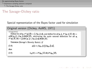
Savage’s density ratio theorem
Given a test H0 : θ = θ0 in a model f (x|θ, ψ) with a nuisance
parameter ψ, under priors π0 (ψ) and π1 (θ, ψ) such that
π1 (ψ|θ0 ) = π0 (ψ)
then
π1 (θ0 |x)
B01 = ,
π1 (θ0 )
with the obvious notations
π1 (θ) = π1 (θ, ψ)dψ , π1 (θ|x) = π1 (θ, ψ|x)dψ ,
[Dickey, 1971; Verdinelli & Wasserman, 1995]

74. On approximating Bayes factors
Importance sampling solutions compared
The Savage–Dickey ratio
Rephrased
“Suppose that f0 (θ) = f1 (θ|φ = φ0 ). As f0 (x|θ) = f1 (x|θ, φ = φ0 ),
Z
f0 (x) = f1 (x|θ, φ = φ0 )f1 (θ|φ = φ0 ) dθ = f1 (x|φ = φ0 ) ,
i.e., the denumerator of the Bayes factor is the value of f1 (x|φ) at φ = φ0 , while the denominator is an average
of the values of f1 (x|φ) for φ = φ0 , weighted by the prior distribution f1 (φ) under the augmented model.
Applying Bayes’ theorem to the right-hand side of [the above] we get
‹
f0 (x) = f1 (φ0 |x)f1 (x) f1 (φ0 )
and hence the Bayes factor is given by
‹ ‹
B = f0 (x) f1 (x) = f1 (φ0 |x) f1 (φ0 ) .
the ratio of the posterior to prior densities at φ = φ0 under the augmented model.”
[O’Hagan & Forster, 1996]

75. On approximating Bayes factors
Importance sampling solutions compared
The Savage–Dickey ratio
Rephrased
“Suppose that f0 (θ) = f1 (θ|φ = φ0 ). As f0 (x|θ) = f1 (x|θ, φ = φ0 ),
Z
f0 (x) = f1 (x|θ, φ = φ0 )f1 (θ|φ = φ0 ) dθ = f1 (x|φ = φ0 ) ,
i.e., the denumerator of the Bayes factor is the value of f1 (x|φ) at φ = φ0 , while the denominator is an average
of the values of f1 (x|φ) for φ = φ0 , weighted by the prior distribution f1 (φ) under the augmented model.
Applying Bayes’ theorem to the right-hand side of [the above] we get
‹
f0 (x) = f1 (φ0 |x)f1 (x) f1 (φ0 )
and hence the Bayes factor is given by
‹ ‹
B = f0 (x) f1 (x) = f1 (φ0 |x) f1 (φ0 ) .
the ratio of the posterior to prior densities at φ = φ0 under the augmented model.”
[O’Hagan & Forster, 1996]

76. On approximating Bayes factors
Importance sampling solutions compared
The Savage–Dickey ratio
Measure-theoretic difficulty
Representation depends on the choice of versions of conditional
densities:
π0 (ψ)f (x|θ0 , ψ) dψ
B01 = [by definition]
π1 (θ, ψ)f (x|θ, ψ) dψdθ
π1 (ψ|θ0 )f (x|θ0 , ψ) dψ π1 (θ0 )
= [specific version of π1 (ψ|θ0 )
π1 (θ, ψ)f (x|θ, ψ) dψdθ π1 (θ0 )
and arbitrary version of π1 (θ0 )]
π1 (θ0 , ψ)f (x|θ0 , ψ) dψ
= [specific version of π1 (θ0 , ψ)]
m1 (x)π1 (θ0 )
π1 (θ0 |x)
= [version dependent]
π1 (θ0 )

77. On approximating Bayes factors
Importance sampling solutions compared
The Savage–Dickey ratio
Measure-theoretic difficulty
Representation depends on the choice of versions of conditional
densities:
π0 (ψ)f (x|θ0 , ψ) dψ
B01 = [by definition]
π1 (θ, ψ)f (x|θ, ψ) dψdθ
π1 (ψ|θ0 )f (x|θ0 , ψ) dψ π1 (θ0 )
= [specific version of π1 (ψ|θ0 )
π1 (θ, ψ)f (x|θ, ψ) dψdθ π1 (θ0 )
and arbitrary version of π1 (θ0 )]
π1 (θ0 , ψ)f (x|θ0 , ψ) dψ
= [specific version of π1 (θ0 , ψ)]
m1 (x)π1 (θ0 )
π1 (θ0 |x)
= [version dependent]
π1 (θ0 )

78. On approximating Bayes factors
Importance sampling solutions compared
The Savage–Dickey ratio
Choice of density version
c Dickey’s (1971) condition is not a condition:
If
π1 (θ0 |x) π0 (ψ)f (x|θ0 , ψ) dψ
=
π1 (θ0 ) m1 (x)
is chosen as a version, then Savage–Dickey’s representation holds

79. On approximating Bayes factors
Importance sampling solutions compared
The Savage–Dickey ratio
Choice of density version
c Dickey’s (1971) condition is not a condition:
If
π1 (θ0 |x) π0 (ψ)f (x|θ0 , ψ) dψ
=
π1 (θ0 ) m1 (x)
is chosen as a version, then Savage–Dickey’s representation holds

80. On approximating Bayes factors
Importance sampling solutions compared
The Savage–Dickey ratio
Savage–Dickey paradox
Verdinelli-Wasserman extension:
π1 (θ0 |x) π1 (ψ|x,θ0 ,x) π0 (ψ)
B01 = E
π1 (θ0 ) π1 (ψ|θ0 )
similarly depends on choices of versions...
...but Monte Carlo implementation relies on specific versions of all
densities without making mention of it
[Chen, Shao & Ibrahim, 2000]

81. On approximating Bayes factors
Importance sampling solutions compared
The Savage–Dickey ratio
Savage–Dickey paradox
Verdinelli-Wasserman extension:
π1 (θ0 |x) π1 (ψ|x,θ0 ,x) π0 (ψ)
B01 = E
π1 (θ0 ) π1 (ψ|θ0 )
similarly depends on choices of versions...
...but Monte Carlo implementation relies on specific versions of all
densities without making mention of it
[Chen, Shao & Ibrahim, 2000]

82. On approximating Bayes factors
Importance sampling solutions compared
The Savage–Dickey ratio
Computational implementation
Starting from the (new) prior
π1 (θ, ψ) = π1 (θ)π0 (ψ)
˜
define the associated posterior
π1 (θ, ψ|x) = π0 (ψ)π1 (θ)f (x|θ, ψ) m1 (x)
˜ ˜
and impose
π1 (θ0 |x)
˜ π0 (ψ)f (x|θ0 , ψ) dψ
=
π0 (θ0 ) m1 (x)
˜
to hold.
Then
π1 (θ0 |x) m1 (x)
˜ ˜
B01 =
π1 (θ0 ) m1 (x)

83. On approximating Bayes factors
Importance sampling solutions compared
The Savage–Dickey ratio
Computational implementation
Starting from the (new) prior
π1 (θ, ψ) = π1 (θ)π0 (ψ)
˜
define the associated posterior
π1 (θ, ψ|x) = π0 (ψ)π1 (θ)f (x|θ, ψ) m1 (x)
˜ ˜
and impose
π1 (θ0 |x)
˜ π0 (ψ)f (x|θ0 , ψ) dψ
=
π0 (θ0 ) m1 (x)
˜
to hold.
Then
π1 (θ0 |x) m1 (x)
˜ ˜
B01 =
π1 (θ0 ) m1 (x)

84. On approximating Bayes factors
Importance sampling solutions compared
The Savage–Dickey ratio
First ratio
If (θ(1) , ψ (1) ), . . . , (θ(T ) , ψ (T ) ) ∼ π (θ, ψ|x), then
˜
1
π1 (θ0 |x, ψ (t) )
˜
T t
converges to π1 (θ0 |x) (if the right version is used in θ0 ).
˜
π1 (θ0 )f (x|θ0 , ψ)
π1 (θ0 |x, ψ) =
˜
π1 (θ)f (x|θ, ψ) dθ

85. On approximating Bayes factors
Importance sampling solutions compared
The Savage–Dickey ratio
Rao–Blackwellisation with latent variables
When π1 (θ0 |x, ψ) unavailable, replace with
˜
T
1
π1 (θ0 |x, z (t) , ψ (t) )
˜
T
t=1
via data completion by latent variable z such that
f (x|θ, ψ) = ˜
f (x, z|θ, ψ) dz
˜
and that π1 (θ, ψ, z|x) ∝ π0 (ψ)π1 (θ)f (x, z|θ, ψ) available in closed
˜
form, including the normalising constant, based on version
π1 (θ0 |x, z, ψ)
˜ ˜
f (x, z|θ0 , ψ)
= .
π1 (θ0 ) ˜
f (x, z|θ, ψ)π1 (θ) dθ

86. On approximating Bayes factors
Importance sampling solutions compared
The Savage–Dickey ratio
Rao–Blackwellisation with latent variables
When π1 (θ0 |x, ψ) unavailable, replace with
˜
T
1
π1 (θ0 |x, z (t) , ψ (t) )
˜
T
t=1
via data completion by latent variable z such that
f (x|θ, ψ) = ˜
f (x, z|θ, ψ) dz
˜
and that π1 (θ, ψ, z|x) ∝ π0 (ψ)π1 (θ)f (x, z|θ, ψ) available in closed
˜
form, including the normalising constant, based on version
π1 (θ0 |x, z, ψ)
˜ ˜
f (x, z|θ0 , ψ)
= .
π1 (θ0 ) ˜
f (x, z|θ, ψ)π1 (θ) dθ

87. On approximating Bayes factors
Importance sampling solutions compared
The Savage–Dickey ratio
Bridge revival (1)
Since m1 (x)/m1 (x) is unknown, apparent failure!
˜
bridge identity
π1 (θ, ψ)f (x|θ, ψ) π1 (ψ|θ) m1 (x)
Eπ1 (θ,ψ|x)
˜
= Eπ1 (θ,ψ|x)
˜
=
π0 (ψ)π1 (θ)f (x|θ, ψ) π0 (ψ) m1 (x)
˜
to (biasedly) estimate m1 (x)/m1 (x) by
˜
T
π1 (ψ (t) |θ(t) )
T
t=1
π0 (ψ (t) )
based on the same sample from π1 .
˜

88. On approximating Bayes factors
Importance sampling solutions compared
The Savage–Dickey ratio
Bridge revival (1)
Since m1 (x)/m1 (x) is unknown, apparent failure!
˜
bridge identity
π1 (θ, ψ)f (x|θ, ψ) π1 (ψ|θ) m1 (x)
Eπ1 (θ,ψ|x)
˜
= Eπ1 (θ,ψ|x)
˜
=
π0 (ψ)π1 (θ)f (x|θ, ψ) π0 (ψ) m1 (x)
˜
to (biasedly) estimate m1 (x)/m1 (x) by
˜
T
π1 (ψ (t) |θ(t) )
T
t=1
π0 (ψ (t) )
based on the same sample from π1 .
˜

89. On approximating Bayes factors
Importance sampling solutions compared
The Savage–Dickey ratio
Bridge revival (2)
Alternative identity
π0 (ψ)π1 (θ)f (x|θ, ψ) π0 (ψ) m1 (x)
˜
Eπ1 (θ,ψ|x) = Eπ1 (θ,ψ|x) =
π1 (θ, ψ)f (x|θ, ψ) π1 (ψ|θ) m1 (x)
¯ ¯
suggests using a second sample (θ(1) , ψ (1) , z (1) ), . . . ,
¯(T ) , ψ (T ) , z (T ) ) ∼ π1 (θ, ψ|x) and the ratio estimate
(θ ¯
T
1 ¯ ¯ ¯
π0 (ψ (t) ) π1 (ψ (t) |θ(t) )
T
t=1
Resulting unbiased estimate:
(t) , ψ (t) ) T ¯
1 t π1 (θ0 |x, z
˜ 1 π0 (ψ (t) )
B01 =
T π1 (θ0 ) T
t=1
π1 (ψ ¯
¯ (t) |θ (t) )

90. On approximating Bayes factors
Importance sampling solutions compared
The Savage–Dickey ratio
Bridge revival (2)
Alternative identity
π0 (ψ)π1 (θ)f (x|θ, ψ) π0 (ψ) m1 (x)
˜
Eπ1 (θ,ψ|x) = Eπ1 (θ,ψ|x) =
π1 (θ, ψ)f (x|θ, ψ) π1 (ψ|θ) m1 (x)
¯ ¯
suggests using a second sample (θ(1) , ψ (1) , z (1) ), . . . ,
¯(T ) , ψ (T ) , z (T ) ) ∼ π1 (θ, ψ|x) and the ratio estimate
(θ ¯
T
1 ¯ ¯ ¯
π0 (ψ (t) ) π1 (ψ (t) |θ(t) )
T
t=1
Resulting unbiased estimate:
(t) , ψ (t) ) T ¯
1 t π1 (θ0 |x, z
˜ 1 π0 (ψ (t) )
B01 =
T π1 (θ0 ) T
t=1
π1 (ψ ¯
¯ (t) |θ (t) )

91. On approximating Bayes factors
Importance sampling solutions compared
The Savage–Dickey ratio
Difference with Verdinelli–Wasserman representation
The above leads to the representation
π1 (θ0 |x) π1 (θ,ψ|x) π0 (ψ)
˜
B01 = E
π1 (θ0 ) π1 (ψ|θ)
which shows how our approach differs from Verdinelli and
Wasserman’s
π1 (θ0 |x) π1 (ψ|x,θ0 ,x) π0 (ψ)
B01 = E
π1 (θ0 ) π1 (ψ|θ0 )

92. On approximating Bayes factors
Importance sampling solutions compared
The Savage–Dickey ratio
Difference with Verdinelli–Wasserman approximation
In terms of implementation,
(t) , ψ (t) ) T ¯
MR 1 t π1 (θ0 |x, z
˜ 1 π0 (ψ (t) )
B01 (x) = ¯ ¯
T π1 (θ0 ) T
t=1
π1 (ψ (t) |θ(t) )
formaly resembles
T T ˜
VW 1 π1 (θ0 |x, z (t) , ψ (t) ) 1 π0 (ψ (t) )
B01 (x) = .
T π1 (θ0 ) T ˜
π1 (ψ (t) |θ0 )
t=1 t=1
But the simulated sequences differ: first average involves
simulations from π1 (θ, ψ, z|x) and from π1 (θ, ψ, z|x), while second
˜
average relies on simulations from π1 (θ, ψ, z|x) and from
π1 (ψ, z|x, θ0 ),

93. On approximating Bayes factors
Importance sampling solutions compared
The Savage–Dickey ratio
Difference with Verdinelli–Wasserman approximation
In terms of implementation,
(t) , ψ (t) ) T ¯
MR 1 t π1 (θ0 |x, z
˜ 1 π0 (ψ (t) )
B01 (x) = ¯ ¯
T π1 (θ0 ) T
t=1
π1 (ψ (t) |θ(t) )
formaly resembles
T T ˜
VW 1 π1 (θ0 |x, z (t) , ψ (t) ) 1 π0 (ψ (t) )
B01 (x) = .
T π1 (θ0 ) T ˜
π1 (ψ (t) |θ0 )
t=1 t=1
But the simulated sequences differ: first average involves
simulations from π1 (θ, ψ, z|x) and from π1 (θ, ψ, z|x), while second
˜
average relies on simulations from π1 (θ, ψ, z|x) and from
π1 (ψ, z|x, θ0 ),

94. On approximating Bayes factors
Importance sampling solutions compared
The Savage–Dickey ratio
Diabetes in Pima Indian women (cont’d)
Comparison of the variation of the Bayes factor approximations
based on 100 replicas for 20, 000 simulations for a simulation from
the above importance, Chib’s, Savage–Dickey’s and bridge
samplers
q
3.4
3.2
3.0
2.8
q
IS Chib Savage−Dickey Bridge

95. On approximating Bayes factors
Nested sampling
Properties of nested sampling
1 Introduction
2 Importance sampling solutions compared
3 Nested sampling
Purpose
Implementation
Error rates
Impact of dimension
Constraints
Importance variant
A mixture comparison
[Chopin & Robert, 2010]

96. On approximating Bayes factors
Nested sampling
Purpose
Nested sampling: Goal
Skilling’s (2007) technique using the one-dimensional
representation:
1
Z = Eπ [L(θ)] = ϕ(x) dx
0
with
ϕ−1 (l) = P π (L(θ) > l).
Note; ϕ(·) is intractable in most cases.

97. On approximating Bayes factors
Nested sampling
Implementation
Nested sampling: First approximation
Approximate Z by a Riemann sum:
j
Z= (xi−1 − xi )ϕ(xi )
i=1
where the xi ’s are either:
deterministic: xi = e−i/N
or random:
x0 = 1, xi+1 = ti xi , ti ∼ Be(N, 1)
so that E[log xi ] = −i/N .

98. On approximating Bayes factors
Nested sampling
Implementation
Extraneous white noise
Take
1 −(1−δ)θ −δθ 1 −(1−δ)θ
Z= e−θ dθ = e e = Eδ e
δ δ
N
1
ˆ
Z= δ −1 e−(1−δ)θi (xi−1 − xi ) , θi ∼ E(δ) I(θi ≤ θi−1 )
N
i=1
N deterministic random
50 4.64 10.5
4.65 10.5
100 2.47 4.9 Comparison of variances and MSEs
2.48 5.02
500 .549 1.01
.550 1.14

99. On approximating Bayes factors
Nested sampling
Implementation
Extraneous white noise
Take
1 −(1−δ)θ −δθ 1 −(1−δ)θ
Z= e−θ dθ = e e = Eδ e
δ δ
N
1
ˆ
Z= δ −1 e−(1−δ)θi (xi−1 − xi ) , θi ∼ E(δ) I(θi ≤ θi−1 )
N
i=1
N deterministic random
50 4.64 10.5
4.65 10.5
100 2.47 4.9 Comparison of variances and MSEs
2.48 5.02
500 .549 1.01
.550 1.14

100. On approximating Bayes factors
Nested sampling
Implementation
Extraneous white noise
Take
1 −(1−δ)θ −δθ 1 −(1−δ)θ
Z= e−θ dθ = e e = Eδ e
δ δ
N
1
ˆ
Z= δ −1 e−(1−δ)θi (xi−1 − xi ) , θi ∼ E(δ) I(θi ≤ θi−1 )
N
i=1
N deterministic random
50 4.64 10.5
4.65 10.5
100 2.47 4.9 Comparison of variances and MSEs
2.48 5.02
500 .549 1.01
.550 1.14

101. On approximating Bayes factors
Nested sampling
Implementation
Nested sampling: Second approximation
Replace (intractable) ϕ(xi ) by ϕi , obtained by
Nested sampling
Start with N values θ1 , . . . , θN sampled from π
At iteration i,
1 Take ϕi = L(θk ), where θk is the point with smallest
likelihood in the pool of θi ’s
2 Replace θk with a sample from the prior constrained to
L(θ) > ϕi : the current N points are sampled from prior
constrained to L(θ) > ϕi .

102. On approximating Bayes factors
Nested sampling
Implementation
Nested sampling: Second approximation
Replace (intractable) ϕ(xi ) by ϕi , obtained by
Nested sampling
Start with N values θ1 , . . . , θN sampled from π
At iteration i,
1 Take ϕi = L(θk ), where θk is the point with smallest
likelihood in the pool of θi ’s
2 Replace θk with a sample from the prior constrained to
L(θ) > ϕi : the current N points are sampled from prior
constrained to L(θ) > ϕi .

103. On approximating Bayes factors
Nested sampling
Implementation
Nested sampling: Second approximation
Replace (intractable) ϕ(xi ) by ϕi , obtained by
Nested sampling
Start with N values θ1 , . . . , θN sampled from π
At iteration i,
1 Take ϕi = L(θk ), where θk is the point with smallest
likelihood in the pool of θi ’s
2 Replace θk with a sample from the prior constrained to
L(θ) > ϕi : the current N points are sampled from prior
constrained to L(θ) > ϕi .

104. On approximating Bayes factors
Nested sampling
Implementation
Nested sampling: Third approximation
Iterate the above steps until a given stopping iteration j is
reached: e.g.,
observe very small changes in the approximation Z;
reach the maximal value of L(θ) when the likelihood is
bounded and its maximum is known;
truncate the integral Z at level , i.e. replace
1 1
ϕ(x) dx with ϕ(x) dx
0

105. On approximating Bayes factors
Nested sampling
Error rates
Approximation error
Error = Z − Z
j 1
= (xi−1 − xi )ϕi − ϕ(x) dx = − ϕ(x) dx
i=1 0 0
j 1
+ (xi−1 − xi )ϕ(xi ) − ϕ(x) dx (Quadrature Error)
i=1
j
+ (xi−1 − xi ) {ϕi − ϕ(xi )} (Stochastic Error)
i=1
[Dominated by Monte Carlo!]

106. On approximating Bayes factors
Nested sampling
Error rates
A CLT for the Stochastic Error
The (dominating) stochastic error is OP (N −1/2 ):
D
N 1/2 {Stochastic Error} → N (0, V )
with
V =− sϕ (s)tϕ (t) log(s ∨ t) ds dt.
s,t∈[ ,1]
[Proof based on Donsker’s theorem]
The number of simulated points equals the number of iterations j,
and is a multiple of N : if one stops at first iteration j such that
e−j/N < , then: j = N − log .

107. On approximating Bayes factors
Nested sampling
Error rates
A CLT for the Stochastic Error
The (dominating) stochastic error is OP (N −1/2 ):
D
N 1/2 {Stochastic Error} → N (0, V )
with
V =− sϕ (s)tϕ (t) log(s ∨ t) ds dt.
s,t∈[ ,1]
[Proof based on Donsker’s theorem]
The number of simulated points equals the number of iterations j,
and is a multiple of N : if one stops at first iteration j such that
e−j/N < , then: j = N − log .

108. On approximating Bayes factors
Nested sampling
Impact of dimension
Curse of dimension
For a simple Gaussian-Gaussian model of dimension dim(θ) = d,
the following 3 quantities are O(d):
1 asymptotic variance of the NS estimator;
2 number of iterations (necessary to reach a given truncation
error);
3 cost of one simulated sample.
Therefore, CPU time necessary for achieving error level e is
O(d3 /e2 )

109. On approximating Bayes factors
Nested sampling
Impact of dimension
Curse of dimension
For a simple Gaussian-Gaussian model of dimension dim(θ) = d,
the following 3 quantities are O(d):
1 asymptotic variance of the NS estimator;
2 number of iterations (necessary to reach a given truncation
error);
3 cost of one simulated sample.
Therefore, CPU time necessary for achieving error level e is
O(d3 /e2 )

110. On approximating Bayes factors
Nested sampling
Impact of dimension
Curse of dimension
For a simple Gaussian-Gaussian model of dimension dim(θ) = d,
the following 3 quantities are O(d):
1 asymptotic variance of the NS estimator;
2 number of iterations (necessary to reach a given truncation
error);
3 cost of one simulated sample.
Therefore, CPU time necessary for achieving error level e is
O(d3 /e2 )

111. On approximating Bayes factors
Nested sampling
Impact of dimension
Curse of dimension
For a simple Gaussian-Gaussian model of dimension dim(θ) = d,
the following 3 quantities are O(d):
1 asymptotic variance of the NS estimator;
2 number of iterations (necessary to reach a given truncation
error);
3 cost of one simulated sample.
Therefore, CPU time necessary for achieving error level e is
O(d3 /e2 )

112. On approximating Bayes factors
Nested sampling
Constraints
Sampling from constr’d priors
Exact simulation from the constrained prior is intractable in most
cases!
Skilling (2007) proposes to use MCMC, but:
this introduces a bias (stopping rule).
if MCMC stationary distribution is unconst’d prior, more and
more difficult to sample points such that L(θ) > l as l
increases.
If implementable, then slice sampler can be devised at the same
cost!
[Thanks, Gareth!]

113. On approximating Bayes factors
Nested sampling
Constraints
Sampling from constr’d priors
Exact simulation from the constrained prior is intractable in most
cases!
Skilling (2007) proposes to use MCMC, but:
this introduces a bias (stopping rule).
if MCMC stationary distribution is unconst’d prior, more and
more difficult to sample points such that L(θ) > l as l
increases.
If implementable, then slice sampler can be devised at the same
cost!
[Thanks, Gareth!]

114. On approximating Bayes factors
Nested sampling
Constraints
Sampling from constr’d priors
Exact simulation from the constrained prior is intractable in most
cases!
Skilling (2007) proposes to use MCMC, but:
this introduces a bias (stopping rule).
if MCMC stationary distribution is unconst’d prior, more and
more difficult to sample points such that L(θ) > l as l
increases.
If implementable, then slice sampler can be devised at the same
cost!
[Thanks, Gareth!]

115. On approximating Bayes factors
Nested sampling
Importance variant
A IS variant of nested sampling
˜
Consider instrumental prior π and likelihood L, weight function
π(θ)L(θ)
w(θ) =
π(θ)L(θ)
and weighted NS estimator
j
Z= (xi−1 − xi )ϕi w(θi ).
i=1
Then choose (π, L) so that sampling from π constrained to
L(θ) > l is easy; e.g. N (c, Id ) constrained to c − θ < r.

116. On approximating Bayes factors
Nested sampling
Importance variant
A IS variant of nested sampling
˜
Consider instrumental prior π and likelihood L, weight function
π(θ)L(θ)
w(θ) =
π(θ)L(θ)
and weighted NS estimator
j
Z= (xi−1 − xi )ϕi w(θi ).
i=1
Then choose (π, L) so that sampling from π constrained to
L(θ) > l is easy; e.g. N (c, Id ) constrained to c − θ < r.

117. On approximating Bayes factors
Nested sampling
A mixture comparison
Benchmark: Target distribution
Posterior distribution on (µ, σ) associated with the mixture
pN (0, 1) + (1 − p)N (µ, σ) ,
when p is known

118. On approximating Bayes factors
Nested sampling
A mixture comparison
Experiment
n observations with
µ = 2 and σ = 3/2,
Use of a uniform prior
both on (−2, 6) for µ
and on (.001, 16) for
log σ 2 .
occurrences of posterior
bursts for µ = xi
computation of the
various estimates of Z

119. On approximating Bayes factors
Nested sampling
A mixture comparison
Experiment (cont’d)
MCMC sample for n = 16 Nested sampling sequence
observations from the mixture. with M = 1000 starting points.

120. On approximating Bayes factors
Nested sampling
A mixture comparison
Experiment (cont’d)
MCMC sample for n = 50 Nested sampling sequence
observations from the mixture. with M = 1000 starting points.

121. On approximating Bayes factors
Nested sampling
A mixture comparison
Comparison
Monte Carlo and MCMC (=Gibbs) outputs based on T = 104
simulations and numerical integration based on a 850 × 950 grid in
the (µ, σ) parameter space.
Nested sampling approximation based on a starting sample of
M = 1000 points followed by at least 103 further simulations from
the constr’d prior and a stopping rule at 95% of the observed
maximum likelihood.
Constr’d prior simulation based on 50 values simulated by random
walk accepting only steps leading to a lik’hood higher than the
bound

122. On approximating Bayes factors
Nested sampling
A mixture comparison
Comparison (cont’d)
q
q
q q
q q
1.15
q q
q
q
q
q q q
q
q
q
1.10
q
q q
q q
q q q
q
q q
q q
q
q q
q q
q
1.05
q
1.00
0.95
q
q
q
q q
q q
q
q q
q
q
q
q
0.90
q
0.85
q
q
q
q
V1
q V2 V3 V4
q
Graph based on a sample of 10 observations for µ = 2 and
σ = 3/2 (150 replicas).