Downloaded 62 times


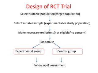

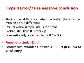
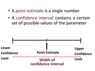
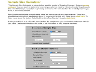
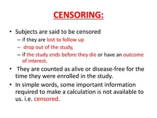
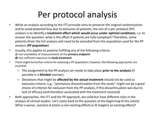
![Significance
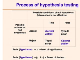
Probability that you reject the null hypothesis (in
favor of the alternative hypothesis) when the
null hypothesis is true:
α = Pr[reject H0 | H0 is true] = Pr[accept H1 | H0
is true]
What does this mean? If we set α = 0.05, then](https://image.slidesharecdn.com/chapter28clincaltrials-191105205115/85/Chapter-28-clincal-trials-34-320.jpg)
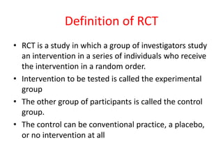
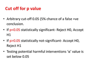
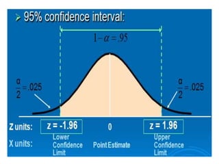
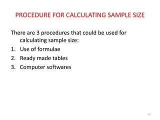
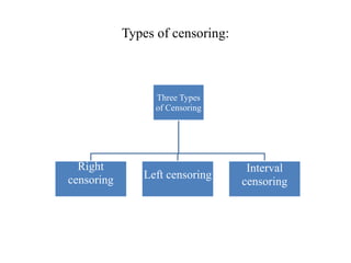
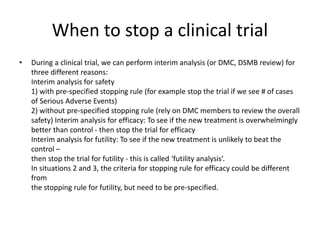
![Power
Probability that you reject the null hypothesis (in
favor of the alternative hypothesis) when the
null hypothesis is false:
1–β = Pr[reject H0 | H1 is true] = Pr[accept H1 |
H1 is true]](https://image.slidesharecdn.com/chapter28clincaltrials-191105205115/85/Chapter-28-clincal-trials-35-320.jpg)


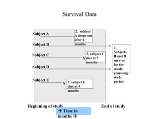

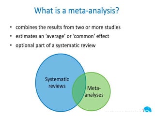


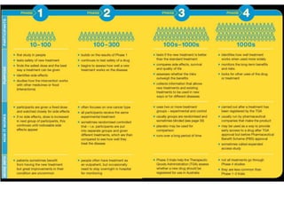
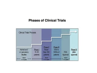
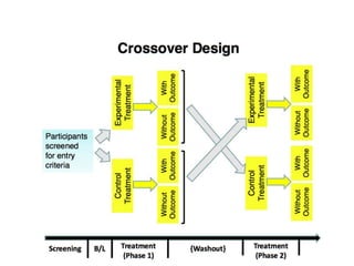
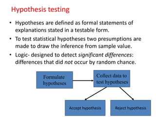
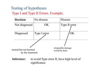
This document provides an overview of clinical trials and their various phases. It discusses how clinical trials are used to test potential interventions in humans to determine if they should be adopted for general use. The different phases of clinical trials are described, including phase I-IV. Key aspects of clinical trial design such as randomization, blinding, and placebos are explained. Hypothesis testing and its role in statistical analysis is also summarized.


![Chapter 39 role of radiotherapy in benign diseases.pptx [read only]](https://cdn.slidesharecdn.com/ss_thumbnails/chapter39roleofradiotherapyinbenigndiseases-191105205437-thumbnail.jpg?width=640&height=640&fit=bounds)


