Download as PDF, PPTX

![Objectives
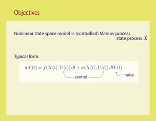
Nonlinear state space model ≡ (controlled) Markov process,
state process X
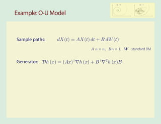
Typical form:
dX(t) = f (X(t), U (t)) dt + σ(X(t), U (t)) dW (t)
noise
control
Questions: For a given feedback law,
• Is the state process stable?
• Is the average cost finite? E[c(X(t), U (t))]
• Can we solve the DP equations? min c(x, u) + Du h∗ (x) = η ∗
u
• Can we approximate the average cost η∗? The value function h∗ ?](https://image.slidesharecdn.com/markovtutorialcdc09-091130151855-phpapp01/85/Markov-Tutorial-CDC-Shanghai-2009-3-320.jpg)
![Outline
Markov Models P t (x, · ) − π f →0
sup Ex [SτC (f )] < ∞
C
π(f ) < ∞
Representations
Lyapunov Theory DV (x) ≤ −f (x) + bIC (x)
Conclusions](https://image.slidesharecdn.com/markovtutorialcdc09-091130151855-phpapp01/85/Markov-Tutorial-CDC-Shanghai-2009-4-320.jpg)
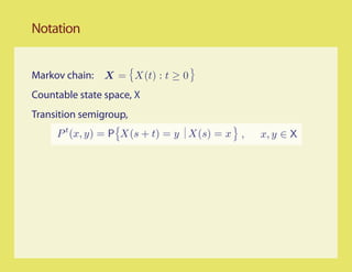
![Notation: Generators & Resolvents
Markov chain: X = X(t) : t ≥ 0
Countable state space, X
Transition semigroup,
P t (x, y) = P X(s + t) = y X(s) = x , x, y ∈ X
Generator: For some domain of functions h,
1
Dh (x) = lim E[h(X(s + t)) − h(X(s)) X(s) = x]
t→0 t
1 t
= lim (P h (x) − h(x))
t→0 t](https://image.slidesharecdn.com/markovtutorialcdc09-091130151855-phpapp01/85/Markov-Tutorial-CDC-Shanghai-2009-7-320.jpg)
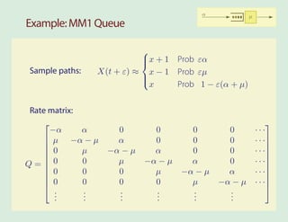
![Notation: Generators & Resolvents
Generator: For some domain of functions h,
1
Dh (x) = lim E[h(X(s + t)) − h(X(s)) X(s) = x]
t→0 t
1 t
= lim (P h (x) − h(x))
t→0 t
Rate matrix:
Dh (x) = Q(x, y)h(y) P t = eQt
y](https://image.slidesharecdn.com/markovtutorialcdc09-091130151855-phpapp01/85/Markov-Tutorial-CDC-Shanghai-2009-8-320.jpg)
![Notation: Generators & Resolvents
Generator: For some domain of functions h,
1
Dh (x) = lim E[h(X(s + t)) − h(X(s)) X(s) = x]
t→0 t
1 t
= lim (P h (x) − h(x))
t→0 t
Rate matrix:
Dh (x) = Q(x, y)h(y) P t = eQt
y
Resolvent:
∞
Rα = e−αt P t
0](https://image.slidesharecdn.com/markovtutorialcdc09-091130151855-phpapp01/85/Markov-Tutorial-CDC-Shanghai-2009-12-320.jpg)
![Notation: Generators & Resolvents
Generator: For some domain of functions h,
1
Dh (x) = lim E[h(X(s + t)) − h(X(s)) X(s) = x]
t→0 t
1 t
= lim (P h (x) − h(x))
t→0 t
Rate matrix:
Dh (x) = Q(x, y)h(y) P t = eQt
y
Resolvent: Resolvent equations:
∞
Rα = e−αt P t Rα = [ Iα − Q]−1
0
QRα = Rα Q = αRα − I](https://image.slidesharecdn.com/markovtutorialcdc09-091130151855-phpapp01/85/Markov-Tutorial-CDC-Shanghai-2009-13-320.jpg)
![Notation: Generators & Resolvents
Motivation: Dynamic programming. For a cost function c,
hα (x) = Rα c (x) = Rα (x, y)c(y)
y∈X
∞
= eαt E[c(X(t)) X(0) = x] dt
0
Discounted-cost value function](https://image.slidesharecdn.com/markovtutorialcdc09-091130151855-phpapp01/85/Markov-Tutorial-CDC-Shanghai-2009-14-320.jpg)
![Notation: Generators & Resolvents
Motivation: Dynamic programming. For a cost function c,
hα (x) = Rα c (x) = Rα (x, y)c(y)
y∈X
∞
= eαt E[c(X(t)) X(0) = x] dt
0
Discounted-cost value function
Resolvent equation = dynamic programming equation,
c + Dhα = αhα](https://image.slidesharecdn.com/markovtutorialcdc09-091130151855-phpapp01/85/Markov-Tutorial-CDC-Shanghai-2009-15-320.jpg)
![Notation: Relative Value Function
Invariant measure π, cost function c , steady-state mean η
Relative value function:
∞
h(x) = E[c(X(t)) − η X(0) = x] dt
0](https://image.slidesharecdn.com/markovtutorialcdc09-091130151855-phpapp01/85/Markov-Tutorial-CDC-Shanghai-2009-18-320.jpg)
![Notation: Relative Value Function
Invariant measure π, cost function c , steady-state mean η
Relative value function:
∞
h(x) = E[c(X(t)) − η X(0) = x] dt
0
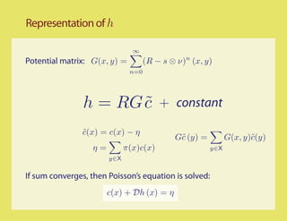
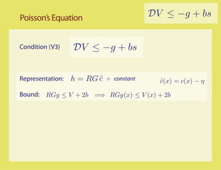
Solution to Poisson’s equation (average-cost DP equation):
c + Dh = η](https://image.slidesharecdn.com/markovtutorialcdc09-091130151855-phpapp01/85/Markov-Tutorial-CDC-Shanghai-2009-19-320.jpg)
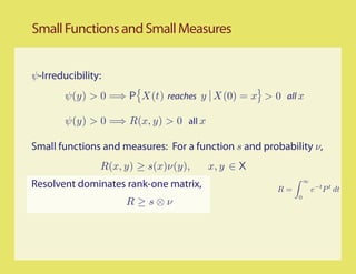
![II
Representations
π ∝ ν[I − (R − s ⊗ ν)]−1
h = [I − (R − s ⊗ ν)]−1 c
˜](https://image.slidesharecdn.com/markovtutorialcdc09-091130151855-phpapp01/85/Markov-Tutorial-CDC-Shanghai-2009-20-320.jpg)

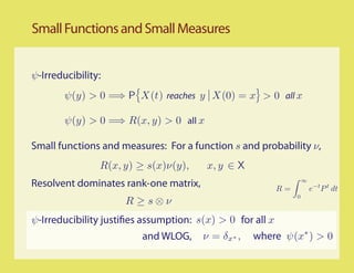

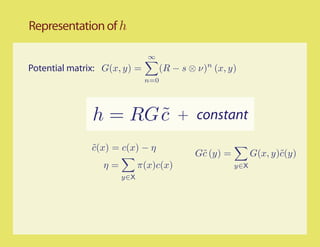
![Potential Matrix
∞
Potential matrix: G(x, y) = (R − s ⊗ ν)n (x, y)
n=0
G = [I − (R − s ⊗ ν)]−1](https://image.slidesharecdn.com/markovtutorialcdc09-091130151855-phpapp01/85/Markov-Tutorial-CDC-Shanghai-2009-27-320.jpg)
![III
Lyapunov Theory
P n (x, · ) − π f →0
sup Ex [SτC (f )] < ∞
C
π(f ) < ∞
∆V (x) ≤ −f (x) + bIC (x)](https://image.slidesharecdn.com/markovtutorialcdc09-091130151855-phpapp01/85/Markov-Tutorial-CDC-Shanghai-2009-31-320.jpg)
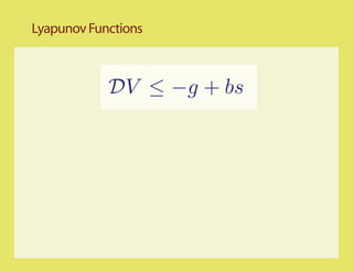
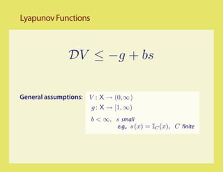
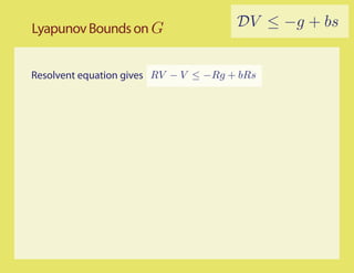
![Lyapunov Bounds on G DV ≤ −g + bs
Resolvent equation gives RV − V ≤ −Rg + bRs
Since s⊗ν is non-negative,
−[I − (R − s ⊗ ν)]V ≤ RV − V ≤ −Rg + bRs
G−1](https://image.slidesharecdn.com/markovtutorialcdc09-091130151855-phpapp01/85/Markov-Tutorial-CDC-Shanghai-2009-35-320.jpg)
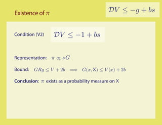
![Lyapunov Bounds on G DV ≤ −g + bs
Resolvent equation gives RV − V ≤ −Rg + bRs
Since s⊗ν is non-negative,
−[I − (R − s ⊗ ν)]V ≤ RV − V ≤ −Rg + bRs
G−1
More positivity, V ≥ GRg − bGRs
Some algebra, GR = G(R − s ⊗ ν) + (Gs) ⊗ ν ≥ G − I
Gs ≤ 1](https://image.slidesharecdn.com/markovtutorialcdc09-091130151855-phpapp01/85/Markov-Tutorial-CDC-Shanghai-2009-36-320.jpg)
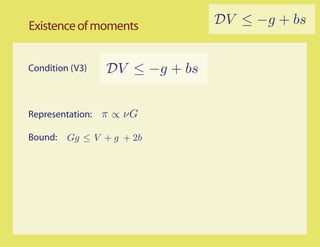
![Lyapunov Bounds on G DV ≤ −g + bs
Resolvent equation gives RV − V ≤ −Rg + bRs
Since s⊗ν is non-negative,
−[I − (R − s ⊗ ν)]V ≤ RV − V ≤ −Rg + bRs
G−1
More positivity, V ≥ GRg − bGRs
Some algebra, GR = G(R − s ⊗ ν) + (Gs) ⊗ ν ≥ G − I
Gs ≤ 1
General bound: GRg ≤ V + 2b
Gg ≤ V + g + 2b](https://image.slidesharecdn.com/markovtutorialcdc09-091130151855-phpapp01/85/Markov-Tutorial-CDC-Shanghai-2009-37-320.jpg)

![P t (x, · ) − π f →0
sup Ex [SτC (f )] < ∞
C
Final words
π(f ) < ∞
DV (x) ≤ −f (x) + bIC (x)
Just as in linear systems theory, Lyapunov functions
provide a characterization of system properties, as well
as a practical verification tool](https://image.slidesharecdn.com/markovtutorialcdc09-091130151855-phpapp01/85/Markov-Tutorial-CDC-Shanghai-2009-51-320.jpg)
![P t (x, · ) − π f →0
sup Ex [SτC (f )] < ∞
C
Final words
π(f ) < ∞
DV (x) ≤ −f (x) + bIC (x)
Just as in linear systems theory, Lyapunov functions
provide a characterization of system properties, as well
as a practical verification tool
Much is left out of this survey - in particular,
• Converse theory
• Limit theory
• Approximation techniques to construct Lyapunov functions
or approximations to value functions
• Application to controlled Markov processes, and
approximate dynamic programming](https://image.slidesharecdn.com/markovtutorialcdc09-091130151855-phpapp01/85/Markov-Tutorial-CDC-Shanghai-2009-52-320.jpg)
![References
[1,4] ψ-Irreducible foundations
[2,11,12,13] Mean- eld models, ODE models, and Lyapunov functions
[1,4,5,9,10] Operator-theoretic methods. See also appendix of [2]
[3,6,7,10] Generators and continuous time models
[1] S. P. Meyn and R. L. Tweedie. Markov chains and stochastic [9] I. Kontoyiannis and S. P. Meyn. Spectral theory and limit
stability. Cambridge University Press, Cambridge, second theorems for geometrically ergodic Markov processes. Ann.
edition, 2009. Published in the Cambridge Mathematical Appl. Probab., 13:304–362, 2003. Presented at the INFORMS
Library. Applied Probability Conference, NYC, July, 2001.
[2] S. P. Meyn. Control Techniques for Complex Networks. Cam- [10] I. Kontoyiannis and S. P. Meyn. Large deviations asymptotics
bridge University Press, Cambridge, 2007. Pre-publication and the spectral theory of multiplicatively regular Markov
edition online: http://black.csl.uiuc.edu/˜meyn. processes. Electron. J. Probab., 10(3):61–123 (electronic),
[3] S. N. Ethier and T. G. Kurtz. Markov Processes : Charac- 2005.
terization and Convergence. John Wiley & Sons, New York, [11] W. Chen, D. Huang, A. Kulkarni, J. Unnikrishnan, Q. Zhu,
1986. P. Mehta, S. Meyn, and A. Wierman. Approximate dynamic
[4] E. Nummelin. General Irreducible Markov Chains and Non- programming using fluid and diffusion approximations with
negative Operators. Cambridge University Press, Cambridge, applications to power management. Accepted for inclusion in
1984. the 48th IEEE Conference on Decision and Control, December
[5] S. P. Meyn and R. L. Tweedie. Generalized resolvents 16-18 2009.
and Harris recurrence of Markov processes. Contemporary [12] P. Mehta and S. Meyn. Q-learning and Pontryagin’s Minimum
Mathematics, 149:227–250, 1993. Principle. Accepted for inclusion in the 48th IEEE Conference
[6] S. P. Meyn and R. L. Tweedie. Stability of Markovian on Decision and Control, December 16-18 2009.
processes III: Foster-Lyapunov criteria for continuous time [13] G. Fort, S. Meyn, E. Moulines, and P. Priouret. ODE
processes. Adv. Appl. Probab., 25:518–548, 1993. methods for skip-free Markov chain stability with applications
[7] D. Down, S. P. Meyn, and R. L. Tweedie. Exponential to MCMC. Ann. Appl. Probab., 18(2):664–707, 2008.
and uniform ergodicity of Markov processes. Ann. Probab.,
23(4):1671–1691, 1995.
[8] P. W. Glynn and S. P. Meyn. A Liapounov bound for solutions
of the Poisson equation. Ann. Probab., 24(2):916–931, 1996.
See also earlier seminal work by Hordijk, Tweedie, ... full references in [1].](https://image.slidesharecdn.com/markovtutorialcdc09-091130151855-phpapp01/85/Markov-Tutorial-CDC-Shanghai-2009-53-320.jpg)

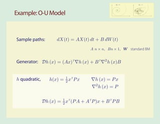
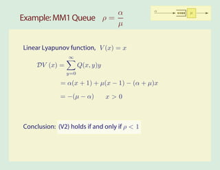
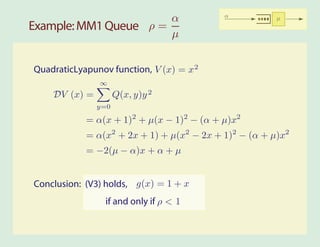
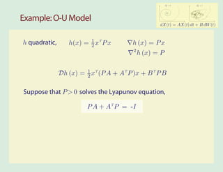
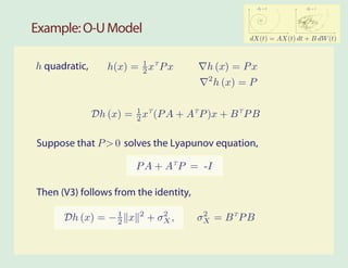
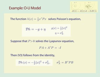
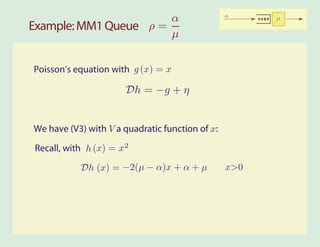
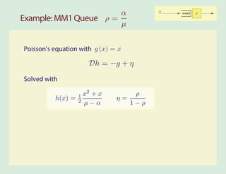
The document discusses the application of Lyapunov functions in the context of Markov processes and dynamic programming, focusing on stability, average cost, and solution methods for dynamic programming equations. It explores various examples such as the MM1 queue and the Ornstein-Uhlenbeck model to illustrate key concepts related to rate matrices, generators, and resolvent equations. The conclusions emphasize the existence of steady-state distributions and the conditions required for moments to be finite.


![11.[104 111]analytical solution for telegraph equation by modified of sumudu ...](https://cdn.slidesharecdn.com/ss_thumbnails/11-104-111analyticalsolutionfortelegraphequationbymodifiedofsumudutransformelzakitransform-120513000219-phpapp01-thumbnail.jpg?width=640&height=640&fit=bounds)


![Lyapunov Stability Rizki Adi Nugroho [1410501075]](https://cdn.slidesharecdn.com/ss_thumbnails/lyapunovstability-rizkiadinugroho1410501075-161123102745-thumbnail.jpg?width=640&height=640&fit=bounds)