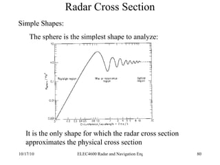
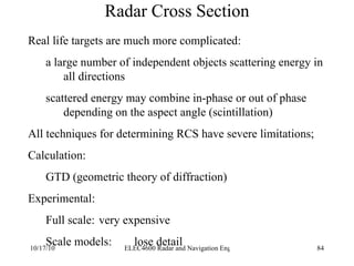
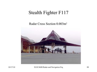
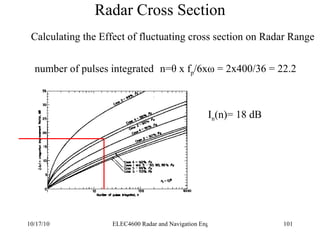
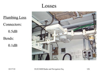
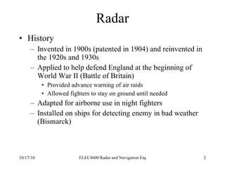
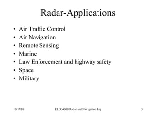
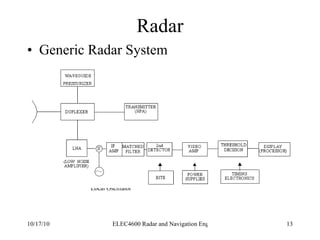
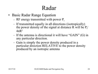
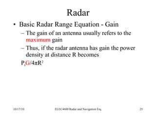
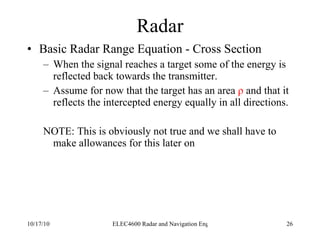
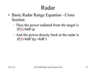
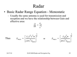
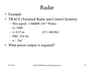
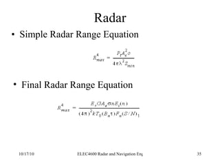
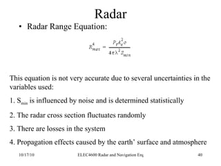
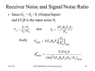
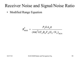
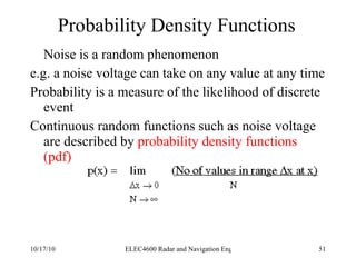
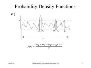
Radar was invented in the early 1900s and applied during World War II to detect aircraft. The basic principles of radar involve transmitting electromagnetic signals that are reflected off targets and detected. A typical radar system includes a transmitter, antenna, receiver, and display. The radar range equation relates key variables such as transmitted power, antenna gain, target radar cross-section, and noise power to determine maximum detection range.

![Radar Basic Radar Range Equation - Maximum Range The radar antenna has a effective are A e and thus the power passed on to the receiver is P r = (P t G /4 π R 2 )( ρ /4 π R 2 ) A e The minimum signal detectable by the receiver is S min and this occurs at the maximum range R MAX Thus S min = (P t G /4 π R MAX 2 )( ρ /4 π R MAX 2 ) A e or R MAX =[P t G A e /(4 π) 2 S min ] ¼](https://image.slidesharecdn.com/radarsurvbw-1232267772428796-3-101017000044-phpapp01/85/Radarsurvbw-1232267772428796-3-28-320.jpg)
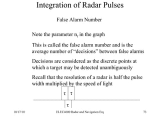
![Integration of Radar Pulses False Alarm Number Thus the total number of unambiguous targets for each transmitted pulse is T/ τ where T is the pulse repetition period (1/f P ) We multiply this by the number of pulses per second (f P ) to get the number of decisions per second Finally we multiply by the False alarm rate (T fa ) to get the number of decisions per false alarm. n f = [ T/ τ][f P ][T fa ]](https://image.slidesharecdn.com/radarsurvbw-1232267772428796-3-101017000044-phpapp01/85/Radarsurvbw-1232267772428796-3-74-320.jpg)
![Integration of Radar Pulses False Alarm Number But T x f P =1 and τ 1/B where B is the IF bandwidth so n f T fa B 1/P fa n f = [ T/ τ][f P ][T fa ]](https://image.slidesharecdn.com/radarsurvbw-1232267772428796-3-101017000044-phpapp01/85/Radarsurvbw-1232267772428796-3-75-320.jpg)