Prof. David Jenn
Departmentof Electrical & Computer Engineering
833 Dyer Road, Room 437
Monterey, CA 93943
(831) 656-2254
jenn@nps.navy.mil, jenn@nps.edu
http://www.nps.navy.mil/faculty/jenn
Radar Fundamentals
2.
2
Overview
• Introduction
• Radarfunctions
• Antennas basics
• Radar range equation
• System parameters
• Electromagnetic waves
• Scattering mechanisms
• Radar cross section and stealth
• Sample radar systems
3.
3
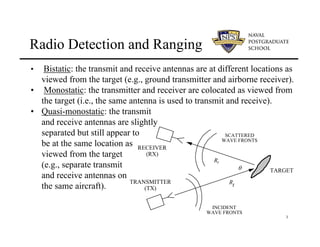
• Bistatic: thetransmit and receive antennas are at different locations as
viewed from the target (e.g., ground transmitter and airborne receiver).
• Monostatic: the transmitter and receiver are colocated as viewed from
the target (i.e., the same antenna is used to transmit and receive).
• Quasi-monostatic: the transmit
and receive antennas are slightly
separated but still appear to
be at the same location as
viewed from the target
(e.g., separate transmit
and receive antennas on
the same aircraft).
Radio Detection and Ranging
TARGET
TRANSMITTER
(TX)
RECEIVER
(RX)
INCIDENT
WAVE FRONTS
SCATTERED
WAVE FRONTS
Rt
Rr
θ
4.
4
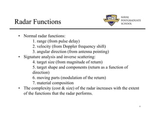
Radar Functions
• Normalradar functions:
1. range (from pulse delay)
2. velocity (from Doppler frequency shift)
3. angular direction (from antenna pointing)
• Signature analysis and inverse scattering:
4. target size (from magnitude of return)
5. target shape and components (return as a function of
direction)
6. moving parts (modulation of the return)
7. material composition
• The complexity (cost & size) of the radar increases with the extent
of the functions that the radar performs.
5.
5
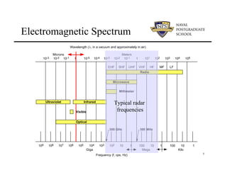
Electromagnetic Spectrum
Wavelength (λ,in a vacuum and approximately in air)
10-3 10-2 10-1 1 10-5 10-4 10-3 10-2 10-1 1 101 102 103 104 105
109 108 107 106 105 104 103 102 10 1 100 10 1 100 10 1
Frequency (f, cps, Hz)
Radio
Microns Meters
Giga Mega Kilo
Microwave
Millimeter
Infrared
Ultraviolet
Visible
Optical
300 MHz
300 GHz
EHF SHF UHF VHF HF MF LF
Typical radar
frequencies
6.
6
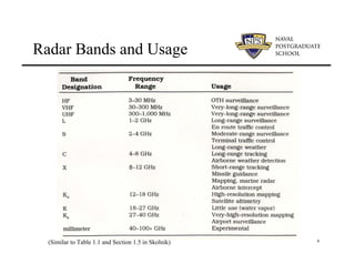
Radar Bands andUsage
8
(Similar to Table 1.1 and Section 1.5 in Skolnik)
7.
7
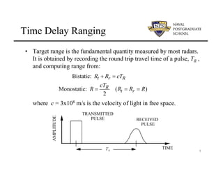
Time Delay Ranging
•Target range is the fundamental quantity measured by most radars.
It is obtained by recording the round trip travel time of a pulse, TR ,
and computing range from:
where c = 3x10⁸ m/s is the velocity of light in free space.
TIME
TR
AMPLITUDE
TRANSMITTED
PULSE RECEIVED
PULSE
Bistatic: t r R
R R cT
+ =
Monostatic: ( )
2
R
t r
cT
R R R R
= = =
8.
8
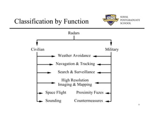
Classification by Function
Radars
CivilianMilitary
Weather Avoidance
Navagation & Tracking
Search & Surveillance
Space Flight
Sounding
High Resolution
Imaging & Mapping
Proximity Fuzes
Countermeasures
9.
9
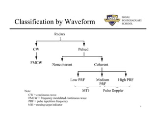
Classification by Waveform
Radars
CWPulsed
Noncoherent Coherent
Low PRF Medium
PRF
High PRF
FMCW
("Pulse doppler")
CW = continuous wave
FMCW = frequency modulated continuous wave
PRF = pulse repetition frequency
Note: MTI Pulse Doppler
MTI = moving target indicator
10.
10
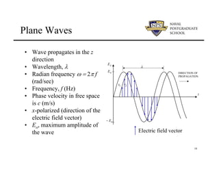
Plane Waves
z
1
t 2
t
x
E
DIRECTIONOF
PROPAGATION
o
E
o
E
−
λ
• Wave propagates in the z
direction
• Wavelength, λ
• Radian frequency ω = 2π f
(rad/sec)
• Frequency, f (Hz)
• Phase velocity in free space
is c (m/s)
• x-polarized (direction of the
electric field vector)
• Eo, maximum amplitude of
the wave Electric field vector
11.
11
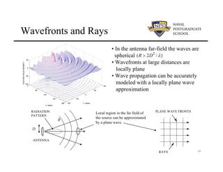
Wavefronts and Rays
•In the antenna far-field the waves are
spherical
• Wavefronts at large distances are
locally plane
• Wave propagation can be accurately
modeled with a locally plane wave
approximation
PLANE WAVE FRONTS
RAYS
Local region in the far field of
the source can be approximated
by a plane wave
ANTENNA
RADIATION
PATTERN
D
R
2
( 2 / )
R D λ
>
12.
12
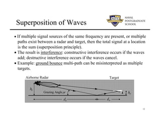
• If multiplesignal sources of the same frequency are present, or multiple
paths exist between a radar and target, then the total signal at a location
is the sum (superposition principle).
• The result is interference: constructive interference occurs if the waves
add; destructive interference occurs if the waves cancel.
• Example: ground bounce multi-path can be misinterpreted as multiple
targets.
Superposition of Waves
t
h
r
h
r
d
t
d
Grazing Angle,ψ
Airborne Radar Target
13.
13
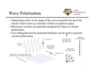
• Polarization refersto the shape of the curve traced by the tip of the
electric field vector as a function of time at a point in space.
• Microwave systems are generally designed for linear or circular
polarization.
• Two orthogonal linearly polarized antennas can be used to generate
circular polarization.
Wave Polarization
1
2
3
4
5
6
LINEAR
POLARIZATION
ELECTRIC FIELD
VECTOR AT AN
INSTANT IN TIME
ORTHOGANAL
TRANSMITTING
ANTENNAS
ELECTRIC
FIELDS
HORIZONTAL, H
VERTICAL, V
HORIZONTAL ANTENNA RECEIVES ONLY
HORIZONTALLY POLARIZED RADIATION
1
2
3
4
CIRCULAR
POLARIZATION
14.
14
Antenna Parameters
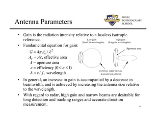
• Gainis the radiation intensity relative to a lossless isotropic
reference.
• Fundamental equation for gain:
• In general, an increase in gain is accompanied by a decrease in
beamwidth, and is achieved by increasing the antenna size relative
to the wavelength.
• With regard to radar, high gain and narrow beams are desirable for
long detection and tracking ranges and accurate direction
measurement.
2
4 /
, effective area
= aperture area
efficiency (0 1)
/ , wavelength
e
e
G A
A A
A
c f
π λ
ε
ε ε
λ
=
=
= ≤ ≤
=
Low gain High gain
(Small in wavelengths) (Large in wavelengths)
ANTENNA DIRECTIONAL
RADIATION PATTERN
Aperture area
15.
15
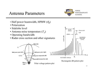
• Half powerbeamwidth, HPBW (θB)
• Polarization
• Sidelobe level
• Antenna noise temperature (TA)
• Operating bandwidth
• Radar cross section and other signatures
Antenna Parameters
0
MAXIMUM
SIDELOBE
LEVEL
PEAK GAIN
GAIN
(dB)
θs
PATTERN ANGLE
θ
SCAN
ANGLE
HPBW
3 dB
0
MAXIMUM
SIDELOBE
LEVEL
PEAK GAIN
GAIN
(dB)
θs
PATTERN ANGLE
θ
SCAN
ANGLE
HPBW
3 dB
Rectangular dB pattern plot
G
0.5G
G
0.5G
Polar voltage pattern plot
16.
16
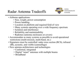
• Airborne applications:
>Size, weight, power consumption
> Power handling
> Location on platform and required field of view
> Many systems operating over a wide frequency spectrum
> Isolation and interference
> Reliability and maintainability
> Radomes (antenna enclosures or covers)
• Accommodate as many systems as possible to avoid operational
restrictions (multi-mission, multi-band, etc.)
• Signatures must be controlled: radar cross section (RCS), infrared
(IR), acoustic, and visible (camouflage)
• New antenna architectures and technologies
> Conformal, integrated
> Digital “smart” antennas with multiple beams
> Broadband
Radar Antenna Tradeoffs
17.
17
Radar Range Equation
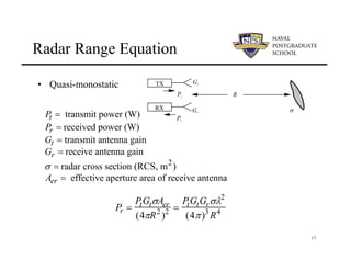
•Quasi-monostatic
2
transmit power (W)
received power (W)
transmit antenna gain
receive antenna gain
radar cross section (RCS, m )
effective aperture area of receive antenna
t
r
t
r
er
P
P
G
G
A
σ
=
=
=
=
=
=
R
TX
Pt
Gt
RX
Pr
Gr σ
Pr =
PtGtσAer
(4πR2
)2 =
PtGtGrσλ2
(4π)3
R4
18.
18
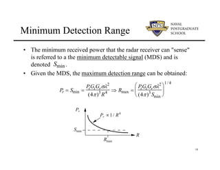
Minimum Detection Range
•The minimum received power that the radar receiver can "sense"
is referred to a the minimum detectable signal (MDS) and is
denoted .
• Given the MDS, the maximum detection range can be obtained:
Smin
R
Pr
Pr ∝1/ R4
Rmax
Smin
Pr = Smin =
PtGtGrσλ2
(4π)3
R4 ⇒ Rmax =
PtGtGrσλ2
(4π)3
Smin
⎛
⎝
⎜
⎞
⎠
⎟
1/4
19.
19
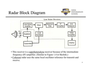
Radar Block Diagram
•This receiver is a superheterodyne receiver because of the intermediate
frequency (IF) amplifier. (Similar to Figure 1.4 in Skolnik.)
• Coherent radar uses the same local oscillator reference for transmit and
receive.
20.
20
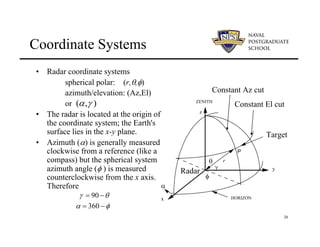
Coordinate Systems
• Radarcoordinate systems
spherical polar: (r,θ,φ)
azimuth/elevation: (Az,El)
or
• The radar is located at the origin of
the coordinate system; the Earth's
surface lies in the x-y plane.
• Azimuth (α) is generally measured
clockwise from a reference (like a
compass) but the spherical system
azimuth angle (φ ) is measured
counterclockwise from the x axis.
Therefore
(α,γ )
α = 360 −φ
γ = 90 −θ
CONSTANT
ELEVATION
x
y
z
θ
φ
γ
ZENITH
HORIZON
P
α
r
Target
Constant El cut
Constant Az cut
Radar
21.
21
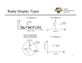
Radar Display Types
RANGE(TIME)
RECEIVED
POWER
TARGET
RETURN
AZIMUTH
RANGE
0
-180 180
TARGET
BLIP
"A" DISPLAY "B" DISPLAY
"C" DISPLAY
PLAN POSITION
INDICATOR (PPI)
AZIMUTH
ELEVATION
0
-180 180
TARGET
BLIP
0
90
RANGE
UNITS
RADAR AT
CENTER
AZIMUTH
TARGET
BLIP
22.
22
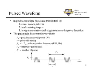
Pulsed Waveform
• Inpractice multiple pulses are transmitted to:
1. cover search patterns
2. track moving targets
3. integrate (sum) several target returns to improve detection
• The pulse train is a common waveform
TIME
τ
Po
Tp
peak instantaneous power (W)
pulse width (sec)
1/ , pulse repetition frequency (PRF, Hz)
interpulse period (sec)
number of pulses
o
p p
p
P
f T
T
N
τ
=
=
=
=
=
23.
23
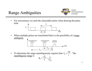
Range Ambiguities
• Forconvenience we omit the sinusoidal carrier when drawing the pulse
train
• When multiple pulses are transmitted there is the possibility of a range
ambiguity.
• To determine the range unambiguously requires that . The
unambiguous range is
TIME
τ
Po
Tp
TIME
TRANSMITTED
PULSE 1
TRANSMITTED
PULSE 2
TARGET
RETURN
TR1
TR2
Tp ≥
2R
c
Ru =
cTp
2
=
c
2 fp
24.
24
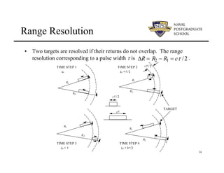
Range Resolution
• Twotargets are resolved if their returns do not overlap. The range
resolution corresponding to a pulse width τ is .
∆R = R2 − R1 = cτ /2
cτ /2
cτ
cτ / 2
TIME STEP 1 TIME STEP 2
TIME STEP 3 TIME STEP 4
to to +τ /2
to + τ to +3τ /2
R1
R2
R1
R1
R1
R2
R2
R2
TARGET
25.
25
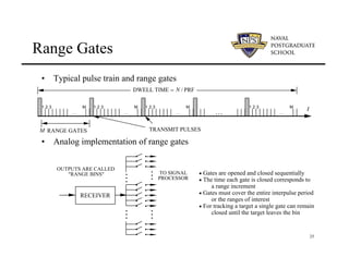
Range Gates
• Typicalpulse train and range gates
• Analog implementation of range gates
L
1 2 3 M
L
1 2 3 M
L
1 2 3 M
L
1 2 3 M
L
DWELL TIME = N / PRF
M RANGE GATES
t
TRANSMIT PULSES
RECEIVER
.
M
M
.
.
.
.
.
.
.
.
.
.
M
M
.
.
.
.
.
.
.
.
.
.
.
TO SIGNAL
PROCESSOR
OUTPUTS ARE CALLED
"RANGE BINS" • Gates are opened and closed sequentially
• The time each gate is closed corresponds to
a range increment
• Gates must cover the entire interpulse period
or the ranges of interest
• For tracking a target a single gate can remain
closed until the target leaves the bin
26.
26
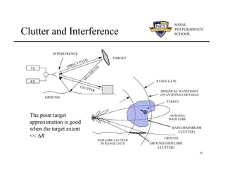
Clutter and Interference
TX
RX
TARGET
GROUND
M
ULTIPA
TH
DIRECTPATH
CLUTTER
INTERFERENCE
ANTENNA
MAIN LOBE
GROUND
SIDELOBE CLUTTER
IN RANGE GATE
RANGE GATE
SPHERICAL WAVEFRONT
(IN ANTENNA FAR FIELD)
TARGET
RAIN (MAINBEAM
CLUTTER)
GROUND (SIDELOBE
CLUTTER)
The point target
approximation is good
when the target extent
<< ∆R
27.
27
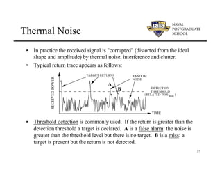
Thermal Noise
• Inpractice the received signal is "corrupted" (distorted from the ideal
shape and amplitude) by thermal noise, interference and clutter.
• Typical return trace appears as follows:
• Threshold detection is commonly used. If the return is greater than the
detection threshold a target is declared. A is a false alarm: the noise is
greater than the threshold level but there is no target. B is a miss: a
target is present but the return is not detected.
TARGET RETURNS
TIME
RECEIVED
POWER
RANDOM
NOISE
DETECTION
THRESHOLD
(RELATED TO S )
min
A
B
28.
28
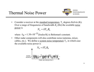
Thermal Noise Power
•Consider a receiver at the standard temperature, To degrees Kelvin (K).
Over a range of frequencies of bandwidth Bn (Hz) the available noise
power is
where (Joules/K) is Boltzman's constant.
• Other radar components will also contribute noise (antenna, mixer,
cables, etc.). We define a system noise temperature Ts, in which case
the available noise power is
No = kTo Bn
23
1.38 10
B
k −
= ×
No = kTsBn
TIME OR FREQUENCY
NOISE
POWER
29.
29
Signal-to-Noise Ratio (SNR)
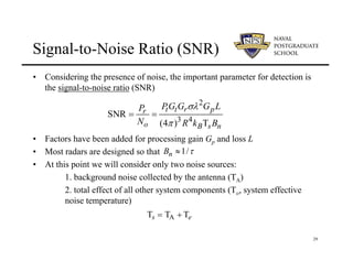
•Considering the presence of noise, the important parameter for detection is
the signal-to-noise ratio (SNR)
• Factors have been added for processing gain Gp and loss L
• Most radars are designed so that
• At this point we will consider only two noise sources:
1. background noise collected by the antenna (TA)
2. total effect of all other system components (To, system effective
noise temperature)
2
3 4
SNR
(4 ) T
t t r p
r
o B s n
PG G G L
P
N R k B
σλ
π
= =
Ts = TA + Te
1/
n
B τ
≈
30.
30
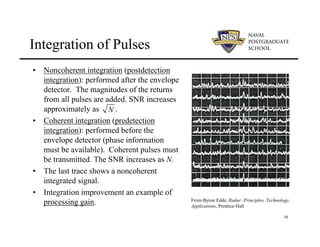
Integration of Pulses
•Noncoherent integration (postdetection
integration): performed after the envelope
detector. The magnitudes of the returns
from all pulses are added. SNR increases
approximately as .
• Coherent integration (predetection
integration): performed before the
envelope detector (phase information
must be available). Coherent pulses must
be transmitted. The SNR increases as N.
• The last trace shows a noncoherent
integrated signal.
• Integration improvement an example of
processing gain.
N
From Byron Edde, Radar: Principles, Technology,
Applications, Prentice-Hall
31.
31
Dwell Time
HALF POWER
ANGLE
HPBW.
.
.
MAXIMUM
VALUE OF
GAIN
ANTENNA POWER
PATTERN (POLAR PLOT)
B
θ
D
B /
λ
θ ≈
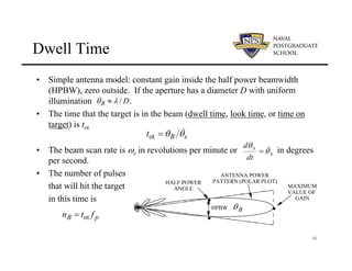
• Simple antenna model: constant gain inside the half power beamwidth
(HPBW), zero outside. If the aperture has a diameter D with uniform
illumination .
• The time that the target is in the beam (dwell time, look time, or time on
target) is tot
• The beam scan rate is ωs in revolutions per minute or in degrees
per second.
• The number of pulses
that will hit the target
in this time is
s
B
t θ
θ &
=
ot
s
s
dt
d
θ
θ &
=
p
B f
t
n ot
=
32.
32
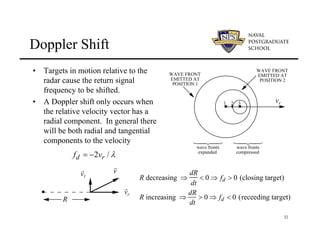
Doppler Shift
• Targetsin motion relative to the
radar cause the return signal
frequency to be shifted.
• A Doppler shift only occurs when
the relative velocity vector has a
radial component. In general there
will be both radial and tangential
components to the velocity
•
• •
1 2 3 vr
wave fronts
expanded
1 2
4 3
4
wave fronts
compressed
1 2
4 3
4
WAVE FRONT
EMITTED AT
POSITION 1
WAVE FRONT
EMITTED AT
POSITION 2
R decreasing ⇒
dR
dt
< 0 ⇒ fd > 0 (closing target)
R increasing ⇒
dR
dt
> 0 ⇒ fd < 0 (receeding target)
r
vt
r
vr
r
v
•
R
2 /
d r
f v λ
= −
33.
33
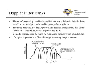
Doppler Filter Banks
•The radar’s operating band is divided into narrow sub-bands. Ideally there
should be no overlap in sub-band frequency characteristics.
• The noise bandwidth of the Doppler filters is small compared to that of the
radar’s total bandwidth, which improves the SNR.
• Velocity estimates can be made by monitoring the power out of each filter.
• If a signal is present in a filter, the target's velocity range is known.
fc
f
fc + fd
AMP FREQUENCY
CHARACTERISTIC
NARROWBAND
DOPPLER FILTERS CROSSOVER
LEVEL
dB
SCALE
34.
34
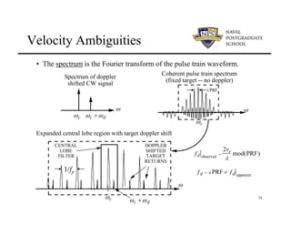
Velocity Ambiguities
ω
ω
ωc ωc+ωd
Spectrum of doppler
shifted CW signal
Coherent pulse train spectrum
(fixed target -- no doppler)
ωc
ωc +ωd
ω
ωc
CENTRAL
LOBE
FILTER fd observed
=
2vr
λ
mod(PRF)
fd = n PRF + fd apparent
Expanded central lobe region with target doppler shift
DOPPLER
SHIFTED
TARGET
RETURNS
• The spectrum is the Fourier transform of the pulse train waveform.
1/PRF
1/fp
35.
35
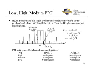
Low, High, MediumPRF
• If fd is increased the true target Doppler shifted return moves out of the
passband and a lower sideband lobe enters. Thus the Doppler measurement
is ambiguous.
• PRF determines Doppler and range ambiguities:
PRF RANGE DOPPLER
High Ambiguous Unambiguous
Medium Ambiguous Ambiguous
Low Unambiguous Ambiguous
ω
ωc +ωd
ωc
APPARENT
DOPPLER
SHIFT
ACTUAL
DOPPLER
SHIFT
fd max = ± f p / 2
vu = λ f dmax / 2
= ±λ f p / 4
∆vu = λ f p / 2
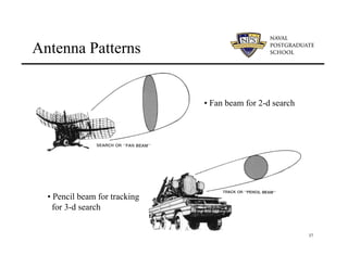
36.
36
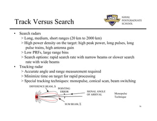
Track Versus Search
•Search radars
> Long, medium, short ranges (20 km to 2000 km)
> High power density on the target: high peak power, long pulses, long
pulse trains, high antenna gain
> Low PRFs, large range bins
> Search options: rapid search rate with narrow beams or slower search
rate with wide beams
• Tracking radar
> Accurate angle and range measurement required
> Minimize time on target for rapid processing
> Special tracking techniques: monopulse, conical scan, beam switching
SUM BEAM, Σ
DIFFERENCE BEAM, ∆
SIGNAL ANGLE
OF ARRIVAL
POINTING
ERROR
SUM BEAM, Σ
DIFFERENCE BEAM, ∆
SIGNAL ANGLE
OF ARRIVAL
POINTING
ERROR
Monopulse
Technique
38
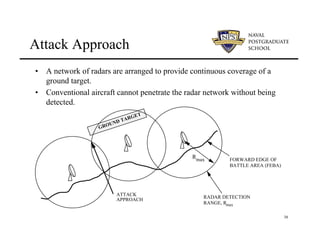
Attack Approach
• Anetwork of radars are arranged to provide continuous coverage of a
ground target.
• Conventional aircraft cannot penetrate the radar network without being
detected.
GROUND TARGET
ATTACK
APPROACH
FORWARD EDGE OF
BATTLE AREA (FEBA)
Rmax
RADAR DETECTION
RANGE, Rmax
39.
39
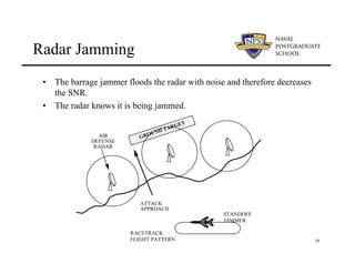
Radar Jamming
• Thebarrage jammer floods the radar with noise and therefore decreases
the SNR.
• The radar knows it is being jammed.
GROUND TARGET
AIR
DEFENSE
RADAR
ATTACK
APPROACH
STANDOFF
JAMMER
RACETRACK
FLIGHT PATTERN
41
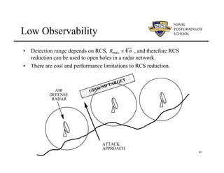
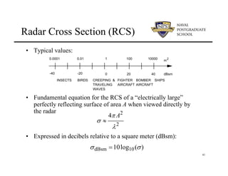
Radar Cross Section(RCS)
• Typical values:
• Fundamental equation for the RCS of a “electrically large”
perfectly reflecting surface of area A when viewed directly by
the radar
• Expressed in decibels relative to a square meter (dBsm):
-40 -20 0 20 40 dBsm
m
2
0.0001 0.01 1 100 10000
INSECTS BIRDS CREEPING &
TRAVELING
WAVES
FIGHTER
AIRCRAFT
BOMBER
AIRCRAFT
SHIPS
2
2
4 A
π
σ
λ
≈
σdBsm =10log10(σ)
42.
42
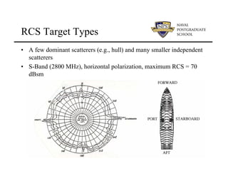
RCS Target Types
•A few dominant scatterers (e.g., hull) and many smaller independent
scatterers
• S-Band (2800 MHz), horizontal polarization, maximum RCS = 70
dBsm
43.
43
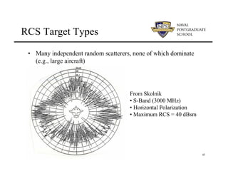
RCS Target Types
•Many independent random scatterers, none of which dominate
(e.g., large aircraft)
From Skolnik
• S-Band (3000 MHz)
• Horizontal Polarization
• Maximum RCS = 40 dBsm
44.
44
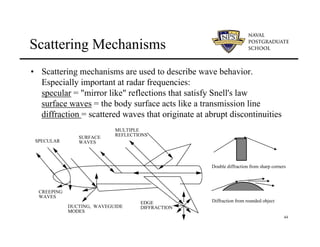
Scattering Mechanisms
Double diffractionfrom sharp corners
Diffraction from rounded object
SPECULAR
DUCTING, WAVEGUIDE
MODES
MULTIPLE
REFLECTIONS
EDGE
DIFFRACTION
SURFACE
WAVES
CREEPING
WAVES
• Scattering mechanisms are used to describe wave behavior.
Especially important at radar frequencies:
specular = "mirror like" reflections that satisfy Snell's law
surface waves = the body surface acts like a transmission line
diffraction = scattered waves that originate at abrupt discontinuities
45.
45
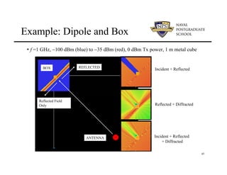
Example: Dipole andBox
• f =1 GHz, −100 dBm (blue) to −35 dBm (red), 0 dBm Tx power, 1 m metal cube
ANTENNA
BOX
Reflected Field
Only
REFLECTED
Incident + Reflected
Reflected + Diffracted
Incident + Reflected
+ Diffracted
ANTENNA
BOX
Reflected Field
Only
REFLECTED
Incident + Reflected
Reflected + Diffracted
Incident + Reflected
+ Diffracted
46.
46
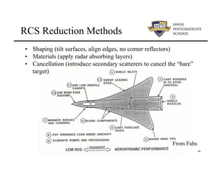
RCS Reduction Methods
•Shaping (tilt surfaces, align edges, no corner reflectors)
• Materials (apply radar absorbing layers)
• Cancellation (introduce secondary scatterers to cancel the “bare”
target)
From Fuhs
47.
47
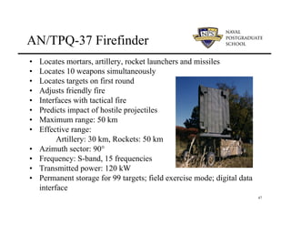
AN/TPQ-37 Firefinder
• Locatesmortars, artillery, rocket launchers and missiles
• Locates 10 weapons simultaneously
• Locates targets on first round
• Adjusts friendly fire
• Interfaces with tactical fire
• Predicts impact of hostile projectiles
• Maximum range: 50 km
• Effective range:
Artillery: 30 km, Rockets: 50 km
• Azimuth sector: 90°
• Frequency: S-band, 15 frequencies
• Transmitted power: 120 kW
• Permanent storage for 99 targets; field exercise mode; digital data
interface