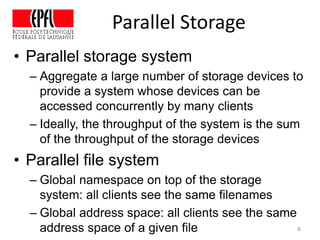
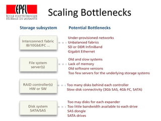
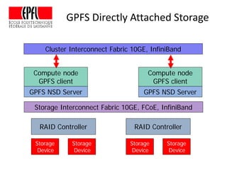
This document discusses storage infrastructure for high-performance computing. It begins by introducing data-intensive science and the need for parallel storage systems. It then discusses several parallel file systems used in HPC like GPFS, Lustre, and PanFS. Key concepts covered include data striping, scale-out NAS, parallel file systems, and IO acceleration techniques. The document also discusses challenges of data growth, bottlenecks in scaling storage, and architectures of various parallel file systems.

1. 1
Storage Infrastructure
for HPC
Gabriel Mateescu
mateescu@acm.org

2. Overview
• Data-intensive science
• Architecture of Parallel Storage
• Parallel File Systems
– GPFS, Lustre, PanFS
• Data Striping
• Scale-out NAS and pNFS
• IO acceleration
2

3. The 4th paradigm of science
• Experiment
• Theory: models
• Computational Science: simulations
• Data-intensive science
– Unifies theory, experiment, and simulation
– Digital information processed by software
– Capture, curation, and analysis of data
– Creates a data explosion effect
3

4. Data Explosion 1
• Explosion of data volume
– The amount of data doubles every two years
– Number of files grows faster
• Challenges:
– Disk bandwidth growth lags compute bandwidth
growth
– Data management: migration to appropriate
performance tier, replication, backup, compression
– Capacity provisioning
4

5. Data Explosion 2
• Turning data into actionable insights
requires solving all these challenges
– Enough storage capacity
– Data placement and migration
– Data transfer bandwidth
– Data discovery
• New technology needed to handle massive
data sizes and file counts
– Access, preservation and movement of data
requires high-performance, scalable storage 5

6. Early days of HPC storage
6
Compute
Node 0
File 0
Local file
system
• One file per compute node
• Hard to manage and data stage-in and stage-
out needed
Compute
Node 1
File 1
Local file
system
Compute
Node 2
File 2
Local file
system
Compute
Node 3
File 3
Local file
system

7. Parallel and shared storage
7
Compute
Node 0
File A
• All compute nodes can access all files
• Multiple compute nodes can access the
same file concurrently
Compute
Node 1
File B
Compute
Node 2
File C
Compute
Node 3
File D
Shared and Parallel File System

8. Parallel Storage
• Parallel storage system
– Aggregate a large number of storage devices to
provide a system whose devices can be
accessed concurrently by many clients
– Ideally, the throughput of the system is the sum
of the throughput of the storage devices
• Parallel file system
– Global namespace on top of the storage
system: all clients see the same filenames
– Global address space: all clients see the same
address space of a given file 8

9. Network Attached Storage
Storage
Device
File System Server
Storage
Device
RAID Controller
Storage
Device
File System Server
Storage
Device
Interconnect Fabric 10GE, InfiniBand
Client node Client node
RAID Controller

10. Directly Attached Storage
Storage
Device
File System Server
Storage Interconnect Fabric 10GE, FCoE, InfiniBand
Storage
Device
Storage
Device
Storage
Device
Cluster Interconnect Fabric 10GE, InfiniBand
Compute node
RAID Controller RAID Controller
File System Server
Compute node

11. Scale-out NAS (SoNAS)
Storage
Device
File System Server
Storage Interconnect Fabric 10GE, FCoE, InfiniBand
Storage
Device
Storage
Device
Storage
Device
WAN Interconnect
Client node
RAID Controller RAID Controller
File System Server
Client node

12. Parallel File System vs SoNAS
• Parallel file system
– Provides high throughput to one file by striping
the file across several storage devices
– Client nodes may also be file system servers
• Scale-out NAS (SoNAS)
– Parallel File System + Parallel Access Protocol
– File system servers typically not on the LAN of
the compute nodes (clients)
12

13. • A LUN is a logical volume made out of
multiple physical disks
• Typically, a LUN is built as a RAID array
– RAID offers redundancy and/or concurrency
• There are several RAID types
– RAID0: striping
– RAID6: striping and two parity blocks
• 8 data disks + 2 parity disks
• Parity disks are distributed across 10 disks
13
LUN and RAID

14. • RAID stripe: a sequence of blocks that
contains one block from each disk of a LUN
– Stripe width = number of disks per LUN
– Stripe depth = size per disk
– Stripe size = Stripe width ×Stripe depth
• File system stripe: a sequence of blocks
(segments) that contains one block from
each LUN
– Stripe width = number of LUNs
– Stripe depth, aka block size
14
Striping

15. Scaling
• Capacity scaling
– cores/node, memory/node, node count
– storage size, network switches
• Performance scaling
– GFlops, Instructions/cycle, Memory bandwidth
– IO throughput: large or small file, metadata
• IO scaling requires a balanced system
architecture to avoid bottlenecks
15

16. Scaling Bottlenecks
16

17. Storage wall
• As the system size (CPUs, memory,
interconnect, the number of compute nodes)
increases, providing scalable IO throughput
becomes very expensive
• Ken Batcher, recipient of the Seymour Cray
award put it this way:
– A supercomputer is a device for turning
compute-bound problems into IO-bound
problems
17

18. IBM GPFS (1)
18
• Global Parallel File System
– Supports both architectures
• network-attached: software or hardware RAID
• directly-attached
– Network Shared Disk
• Cluster-wide naming
• Access to data
– Full POSIX semantics
• Atomicity of concurrent read and write operations

19. GPFS Directly Attached Storage
Storage
Device
Storage Interconnect Fabric 10GE, FCoE, InfiniBand
Storage
Device
Storage
Device
Storage
Device
Cluster Interconnect Fabric 10GE, InfiniBand
RAID Controller RAID Controller
GPFS NSD Server
Compute node
GPFS client
GPFS NSD Server
Compute node
GPFS client

20. GPFS Network Attached Storage
Storage
Device
Storage Node
NSD Server
Storage
Device
Interconnect Fabric 10GE, InfiniBand
Compute node
GPFS client
NSD
Storage
Device
Storage Node
NSD Server
Storage
Device
Compute node
GPFS client
NSD

21. HA for Network Attached Storage
Storage
Array
Storage
Node
Storage
Array
Storage
Node
• If a storage node fails, the load on the other
storage node doubles
• Tolerates failure of one out of two nodes

22. Triad HA
Storage
Array
Storage
Node
Storage
Node
• If a storage node fails, the load on the other
two storage nodes grows with 50%
• Tolerates failure of two out of three nodes
Storage
Node
Storage
Array
Storage
Array

23. IBM GPFS 2
23
• Nodeset: group of nodes that operate on the
same file systems
• GPFS management servers
– cluster data server: one or two per cluster
• cluster configuration and file system information
– file system manager: one per file system
• disk space allocation, token management server
– configuration manager: one per nodeset
• Selects file system manager
– metanode: one per opened file
• handles updates to metadata

24. GPFS Scaling
• GPFS meta-nodes
– Each directory is assigned to a metanode that
manages it, e.g., locking
– Each file is assigned to a metanode that
manages it, e.g., locking
• The meta-node may become a bottleneck
– One file per task: puts pressure on the directory
meta-node for large jobs, unless a directory
hierarchy is created
– One shared file: puts pressure on the file meta-
node for large jobs 24

25. GPFS Striping (1)
• GPFS-level striping: spread the blocks of a
file across all LUNs
– Stripe width = number of LUNs
– GPFS block size = block stored in a LUN
• RAID-level striping
– Assume RAID6 with 8+2P, block-level striping
– Stripe width is 8 (8 + 2P)
– Stripe depth is the size of a block written to one
disk; a multiple of the sector size, e.g., 512 KiB
– Stripe size = Stripe depth × Stripe width = 8 ×
512 KiB = 4 MiB 25

26. GPFS Striping (2)
• GPFS block size
– equal to the RAID stripe size = 4 MiB
• Stripe width impacts aggregate bandwidth
– GPFS Stripe width equal to number of LUNs
maximizes throughout per file
– RAID Stripe Width of 8 (8+2P) for RAID6
balances performance and fault tolerance
• Applications should write blocks that are
– multiple of the GPFS block size and aligned
with the GPFS blocks
26

27. Impact of IO Block Size
27
IO size (Bytes)
Throughput (MB/sec) for a 1TB
SAS Seagate Barracuda ES2 disk

28. Handling Small Files
• Small files do not benefit from GPFS striping
• Techniques used for small files
– Read-ahead: pre-fetch next disk block on disk
– Write behind: buffer writes
• These are used by other parallel file
systems as well
– For example, Panasas PanFS
28

29. Lustre file system 1
• Has the network-attached architecture
• Object-based storage
– Uses storage objects instead of blocks
– Storage objects are units of storage that have
variable size, e.g., an entire data structure or
database table
– File layout gives the placement of objects rather
than blocks
• User can set stripe width and depth,
and the file layout 29

30. Lustre Architecture
Object
Storage
Target
Object Storage
Server (OSS)
Interconnect Fabric 10GE, InfiniBand
Lustre client Lustre client
Metadata Server
(MDS)
Object
Storage
Target
Object
Storage
Target
Object Storage
Server (OSS)
Object
Storage
Target
Metadata Target

31. Lustre file system 2
• Metadata servers (MDS)
– Manages file metadata and global namespace
• Object storage server (OSS)
– Is the software that fulfills requests from clients
and gets/stores data to one or more Object
Storage Targets (OSTs)
– An OST is a logical unit number, which can
consists of one or more disk drives (RAID)
• Management Server (MGS)
– can be co-located with MDS/MDT 31

32. Parallel NFS (pNFS)
• pNFS allows clients to access storage
directly and in parallel
– Separation of data and metadata
– Direct access to the data servers
– Out-of-band metadata access
• Storage access protocols:
– File: NFS v4.1
– Object: object-based storage devices (OSD)
– Block: iSCSI, FCoE
32

33. pNFS architecture
NFS Data Server
pNFS client
NFS MDS
pNFS client
NFS Data Server

34. pNFS over Lustre
NFS Data Server
pNFS client
Lustre MDS
pNFS client
NFS MDS
Lustre OSS
NFS Data Server
Lustre OSS

35. Panasas Solution (1)
• SoNAS based on
– PanFS: Panasas ActiveScale file system
– pNFS or DirectFlow: Parallel access protocol
• Architecture
– Director Blade: MDS and management
– Storage Blade: storage nodes
• Disk: 2 or 3 TB/disk, 75 MB/s, one or two disks
• SSD (some models): 32 GB SLC
• CPU + Cache
– Shelf = 1 director blade + 10 storage blades 35

36. pNFS over PanFS
NFS Data Server
pNFS client
Director Blade
pNFS client
NFS MDS
Storage Blade
NFS Data Server
Storage Blade

37. Panasas Solution (2)
• Feeds and Speeds
– Shelf: 10 storage blades + 1 directory blade
• Disk Size = 10 * 6 TB = 60 TB
• Disk Throughput: 10 * (2 * 75 MB/s) = 1.5 GB/s
– Rack: 10 shelves
• Size = 600 TB
• Throughput: 15 GB/s
– System: 10 racks
• Size = 6 PB
• Throughput: 150 GB/s
37

38. Data vs Computation
Movement
38
• Consider a Lustre cluster with
–100 compute nodes (CNs), each with 1
TB local storage, 80 MB/s per local disk
–10 OSS and 10 OSTs/OSS,
–1TB/OST, 80 MB/s per OST
–4x SDR InfiniBand network, has 8 Gbps
that is, 1 GB/s

39. Lustre cluster
Object
Storage
Target
Object Storage
Server (OSS)
InfiniBand Fabric
Lustre client
Metadata Server
(MDS)
Object
Storage
Target
Object
Storage
Target
Object Storage
Server (OSS)
Object
Storage
Target
Metadata Target
Compute node
Lustre client
Compute node
Local Disk Local Disk
1 GB/s
80 MB/s

40. MapReduce /Lustre
40
• Compute Nodes access data from
Lustre
• Disk throughput per OSS = 10 * 80
MB/s = 800 MB/s
–InfiniBand has 1 GB/s, so it can sustain
this throughput
• Aggregate disk throughput
–10 * 800 MB/s = 8 GB/s

41. MapReduce on Lustre vs
HDFS
41
• MapReduce/HDFS:
– Compute nodes use local disks
– Per compute-node throughput is 80 MB/s
– Aggregate disk throughput is 100 * 80 MB/s =
8 GB/s
• Aggregate throughput is the same, 8 GB/s
– The interconnect fabric provides enough
bandwidth for the disks
• MapReduce/Lustre is competitive with
MapReduce/HDFS for latency-tolerant work

42. Data & Compute Trends
• Compute power: 90% per year
• Data volume: 40-60% per year
• Disk capacity: 50% per year
• Disk bandwidth: 15% per year
• Balancing the compute and disk
throughput requires the number of
disks to grow faster than the number of
compute nodes
42

43. IO Acceleration
43
• Disk bandwidth does not keep up with
memory and network bandwidth
• Hide low disk bandwidth using fast
buffering of IO data
–IO forwarding
–SSDs

44. Data Staging
44
• Data staging
–IO forwarding or SSDs
• IO forwarding hides disk bandwidth by
–Buffering the IO generated by an
application on staging machine: free
memory on the supercomputer for
simulation
– Overlapping computation on the
supercomputer with IO on the staging
machine

45. 45
• Consider a machine with 1 PB of RAM that
reaches the peak performance of 1 PFlop/sec
when the operational intensity is >= 2 Flop/B
• Consider an application with operational intensity
1 Flop/B that uses 1 PB of RAM, executes 600
PFlop/iteration, and dumps each iterate to disk
• Running the application on the above machine
takes a time per iteration
Tcomp = (600 PFlop/iteration )/(.1 PFlop/sec) = 6000 sec
Benefits of IO forwarding (1)

46. Benefits of IO forwarding (2)
46
• We can hide almost all the IO time if we can
– Copy 1PB to a staging machine in Tfwd << Tcomp
– Write the 1 PB from the staging machine to disk in
(Tcomp – Tfwd ) ~ Tcomp
• Assume the staging machine has 64 K nodes
each with a 4x QDR port (4 GB/sec per port); then
Throughput = 64 K * 4 GB/sec = 256 TB/sec
Tfwd = 1024 TB/ (64 K * 4 GB/sec) = 4 sec << Tcomp
• So the required disk bandwidth is
BW = (1 PB) / (6000 sec) = 166 GB/sec << 256 TB/sec
• Similar benefit for SSDs

47. SSD Metadata Store
• MDS is a bottleneck for metadata-
intensive operations
• Use SSD for the metadata store
• IBM GPFS with SSD for metadata store
– eight NSD servers with four 1.8 TB SSD and 1.25
GB/s, PCIe attached; two GPFS clients
– Processes the 6.5 TB of metadata for a file
system with 10 Billion files in 43 min
– Enable timely policy-driven data management
47

48. Conclusion
• Parallel storage has evolved similarly
to parallel computation
– Scale by adding disk drives, networking, CPU,
and memory/cache
• Parallel file systems provide direct and
parallel access to storage
– Striping across and within storage nodes
• Staging to SSDs or another machine
hides the disk bandwidth
48