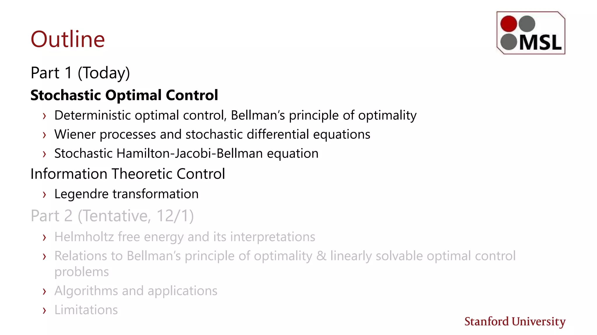
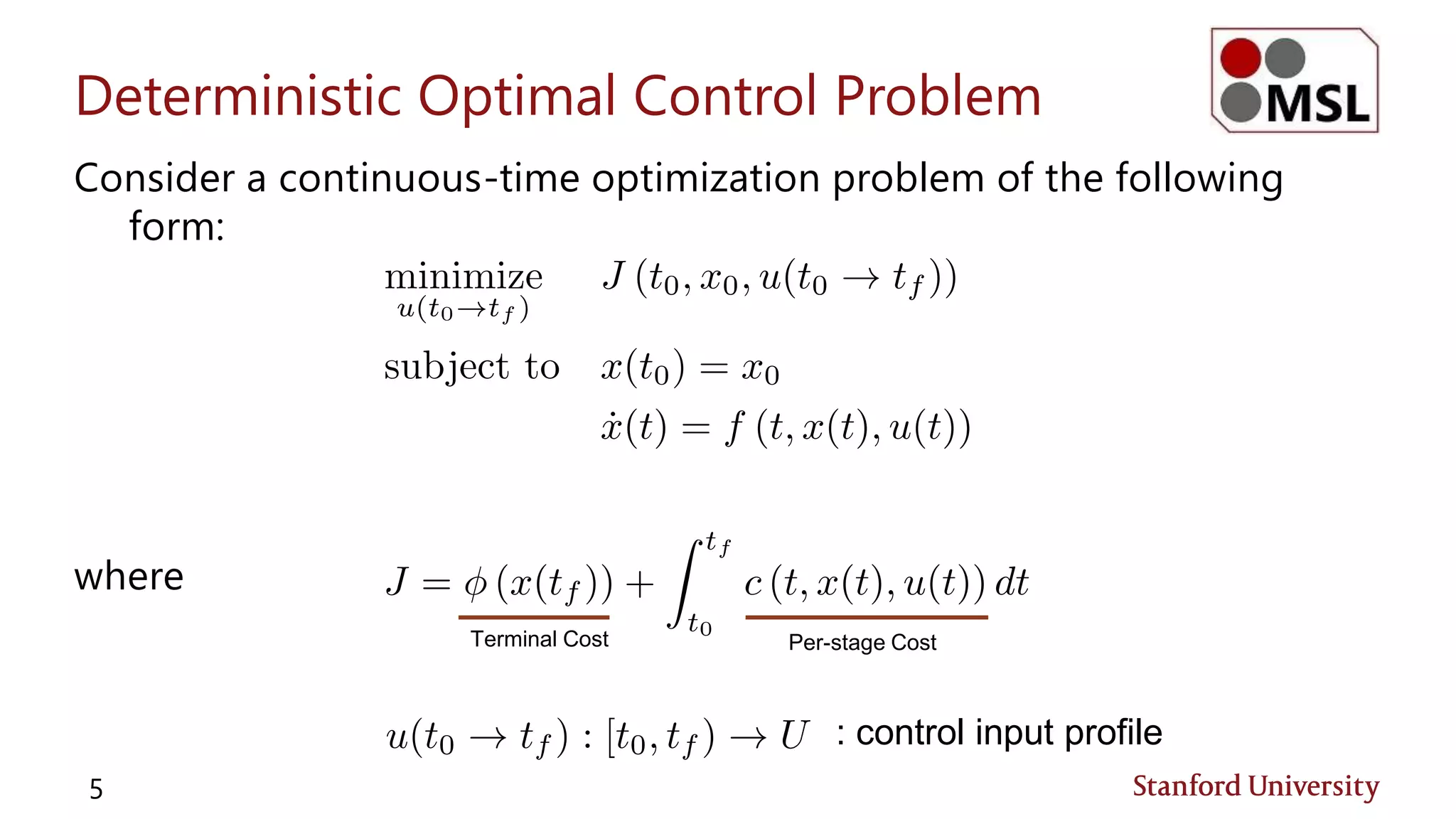
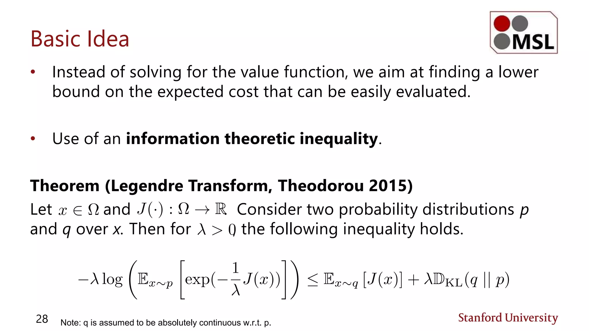
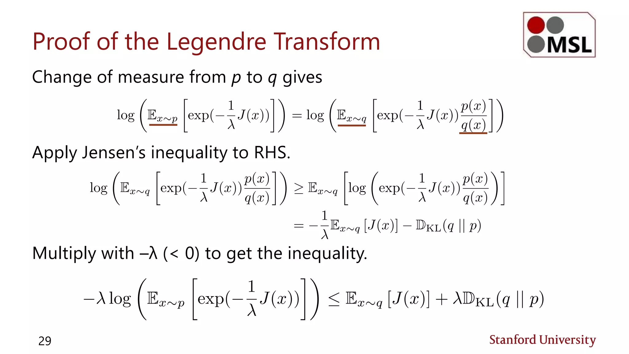
This document discusses stochastic optimal control and information theoretic dualities, highlighting two main approaches: stochastic dynamic programming and forward sampling of stochastic differential equations. It details the Hamilton-Jacobi-Bellman equation and its significance in stochastic control problems, alongside applications in fields such as finance and physics. Additionally, the document examines the Legendre transform as a method for understanding optimal control and its relation to Bellman's principle of optimality.

![The Big Picture
2 [Williams et al., 2017]
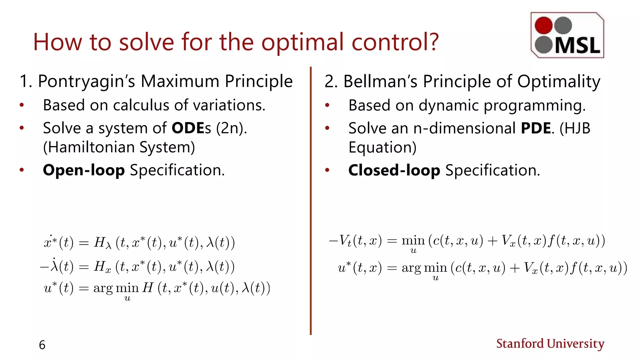
Stochastic Optimal Control Theory
• “Optimality” defined by Bellman’s
principle of optimality.
• Solution methods based on stochastic
dynamic programming.
Information Theoretic Control Theory
• “Optimality” defined in the sense of
Legendre transform.
• Solution methods based on forward
sampling of stochastic differential
equations.
Two fundamentally different approaches to stochastic control problems.](https://image.slidesharecdn.com/socitcdualities-171111051326/75/Stochastic-Optimal-Control-Information-Theoretic-Dualities-2-2048.jpg)
![The Big Picture
3 [Williams et al., 2017]
V(x0) Values of terminal states
x
0
Stochastic Dynamic Programming
Forward Sampling of SDEs
Space of value
function
State space](https://image.slidesharecdn.com/socitcdualities-171111051326/75/Stochastic-Optimal-Control-Information-Theoretic-Dualities-3-2048.jpg)
![Example: The Drunken Spider Problem
Presence of noise (alcohol) can change the optimal behavior
significantly.
11
• Without noise, the spider
will cross the bridge.
• When drunk, the cost of
crossing the bridge
increases and the spider
should go around the lake.
[Kappen, 2005]](https://image.slidesharecdn.com/socitcdualities-171111051326/75/Stochastic-Optimal-Control-Information-Theoretic-Dualities-11-2048.jpg)
![Jensen’s Inequality (Review)
Let f be a convex function over a real-valued random variable X.
Then,
Furthermore, if f is strictly convex, the equality holds if and only if X =
E[X] with probability 1, in which case X is a deterministic constant.
In our case, log() is a strictly concave function, so the direction of the
inequality is flipped.
30](https://image.slidesharecdn.com/socitcdualities-171111051326/75/Stochastic-Optimal-Control-Information-Theoretic-Dualities-30-2048.jpg)