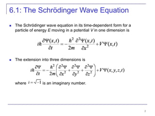
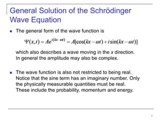
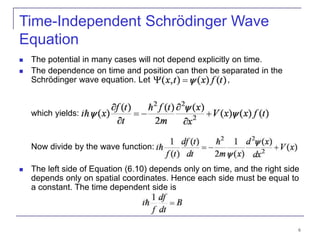
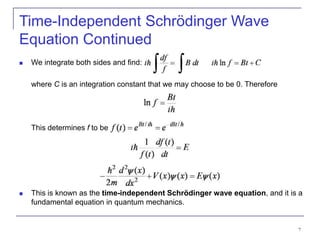
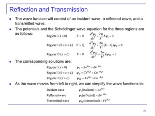
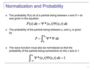
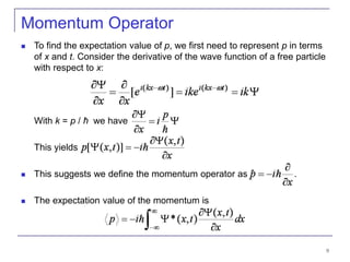
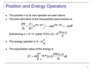
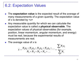
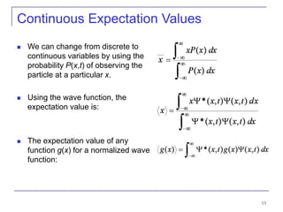
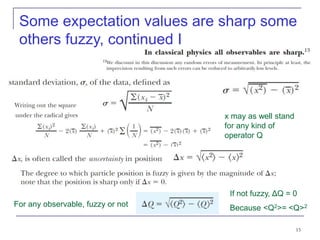
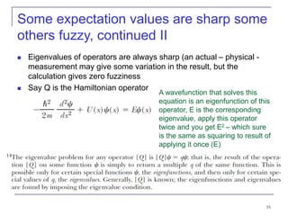
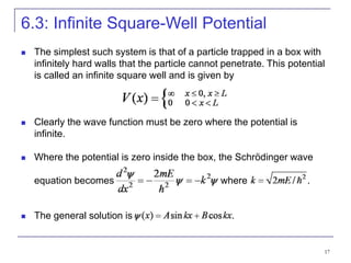
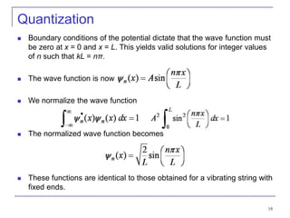
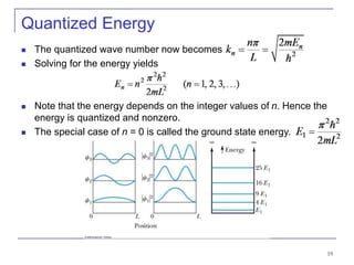
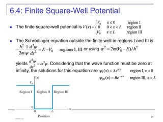
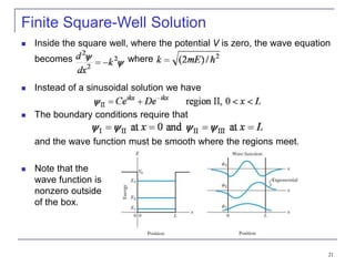
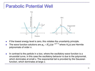
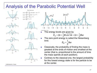
This document provides an overview of quantum mechanics topics including: 1) The Schrödinger wave equation and its time-dependent and time-independent forms. 2) Expectation values and how they are used to calculate probabilities, momentum, position, and energy. 3) Specific quantum systems like infinite and finite square wells and simple harmonic oscillators. It also discusses quantization, degeneracy, and other concepts. 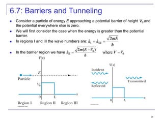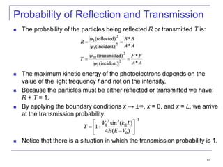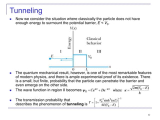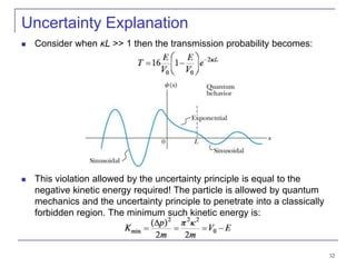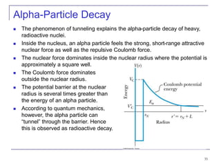4) Barrier penetration and tunneling, where particles can pass through barriers that would be forbidden classically. The document covers many fundamental aspects of quantum mechanics through examining various quantum systems and potentials.

1. 1
 6.1 The Schrödinger Wave Equation
 6.2 Expectation Values
 6.3 Infinite Square-Well Potential
 6.4 Finite Square-Well Potential
 6.5 Three-Dimensional Infinite-Potential Well
 6.6 Simple Harmonic Oscillator
 6.7 Barriers and Tunneling
CHAPTER 6
Quantum Mechanics II
I think it is safe to say that no one understands quantum mechanics. Do
not keep saying to yourself, if you can possibly avoid it, “But how can it
be like that?” because you will get “down the drain” into a blind alley from
which nobody has yet escaped. Nobody knows how it can be like that.
- Richard Feynman

2. 2
6.1: The Schrödinger Wave Equation
 The Schrödinger wave equation in its time-dependent form for a
particle of energy E moving in a potential V in one dimension is
 The extension into three dimensions is
where is an imaginary number.

3. 3
General Solution of the Schrödinger
Wave Equation
 The general form of the wave function is
which also describes a wave moving in the x direction.
In general the amplitude may also be complex.
 The wave function is also not restricted to being real.
Notice that the sine term has an imaginary number. Only
the physically measurable quantities must be real.
These include the probability, momentum and energy.

4. 4
Normalization and Probability
 The probability P(x) dx of a particle being between x and X + dx
was given in the equation
 The probability of the particle being between x1 and x2 is given
by
 The wave function must also be normalized so that the
probability of the particle being somewhere on the x axis is 1.

5. 5
Properties of Valid Wave Functions
Boundary conditions
1) In order to avoid infinite probabilities, the wave function must be finite
everywhere.
2) In order to avoid multiple values of the probability, the wave function
must be single valued.
3) For finite potentials, the wave function and its derivative must be
continuous. This is required because the second-order derivative term
in the wave equation must be single valued. (There are exceptions to
this rule when V is infinite.)
4) In order to normalize the wave functions, they must approach zero as x
approaches infinity.
 Solutions that do not satisfy these properties do not generally
correspond to physically realizable circumstances.

6. 6
Time-Independent Schrödinger Wave
Equation
 The potential in many cases will not depend explicitly on time.
 The dependence on time and position can then be separated in the
Schrödinger wave equation. Let ,
which yields:
Now divide by the wave function:
 The left side of Equation (6.10) depends only on time, and the right side
depends only on spatial coordinates. Hence each side must be equal to
a constant. The time dependent side is

7. 7
 We integrate both sides and find:
where C is an integration constant that we may choose to be 0. Therefore
This determines f to be
 This is known as the time-independent Schrödinger wave equation, and it is a
fundamental equation in quantum mechanics.
Time-Independent Schrödinger Wave
Equation Continued

8. 8
Stationary State
 The wave function can be written as:
 The probability density becomes:
 The probability distributions are constant in time. This is a standing
wave phenomena that is called the stationary state.

9. 9
Momentum Operator
 To find the expectation value of p, we first need to represent p in terms
of x and t. Consider the derivative of the wave function of a free particle
with respect to x:
With k = p / ħ we have
This yields
 This suggests we define the momentum operator as .
 The expectation value of the momentum is

10. 10
 The position x is its own operator as seen above.
 The time derivative of the free-particle wave function is
Substituting ω = E / ħ yields
 The energy operator is
 The expectation value of the energy is
Position and Energy Operators

11. 11
Comparison of Classical and Quantum
Mechanics
 Newton’s second law and Schrödinger’s wave equation are
both differential equations.
 Newton’s second law can be derived from the Schrödinger
wave equation, so the latter is the more fundamental.
 Classical mechanics only appears to be more precise because
it deals with macroscopic phenomena. The underlying
uncertainties in macroscopic measurements are just too small
to be significant.

12. 12
6.2: Expectation Values
 The expectation value is the expected result of the average of
many measurements of a given quantity. The expectation value
of x is denoted by <x>
 Any measurable quantity for which we can calculate the
expectation value is called a physical observable. The
expectation values of physical observables (for example,
position, linear momentum, angular momentum, and energy)
must be real, because the experimental results of
measurements are real.
 The average value of x is

13. 13
Continuous Expectation Values
 We can change from discrete to
continuous variables by using the
probability P(x,t) of observing the
particle at a particular x.
 Using the wave function, the
expectation value is:
 The expectation value of any
function g(x) for a normalized wave
function:

14. 14
Some expectation values are sharp some
others fuzzy
Since there is scatter in the actual positions
(x), the calculated expectation value will
have an uncertainty, fuzziness (Note that x
is its own operator.)

15. 15
Some expectation values are sharp some
others fuzzy, continued I
For any observable, fuzzy or not
If not fuzzy, ΔQ = 0
Because <Q2>= <Q>2
x may as well stand
for any kind of
operator Q

16. 16
Some expectation values are sharp some
others fuzzy, continued II
 Eigenvalues of operators are always sharp (an actual – physical -
measurement may give some variation in the result, but the
calculation gives zero fuzziness
 Say Q is the Hamiltonian operator
A wavefunction that solves this
equation is an eigenfunction of this
operator, E is the corresponding
eigenvalue, apply this operator
twice and you get E2 – which sure
is the same as squaring to result of
applying it once (E)

17. 17
6.3: Infinite Square-Well Potential
 The simplest such system is that of a particle trapped in a box with
infinitely hard walls that the particle cannot penetrate. This potential
is called an infinite square well and is given by
 Clearly the wave function must be zero where the potential is
infinite.
 Where the potential is zero inside the box, the Schrödinger wave
equation becomes where .
 The general solution is .

18. 18
Quantization
 Boundary conditions of the potential dictate that the wave function must
be zero at x = 0 and x = L. This yields valid solutions for integer values
of n such that kL = nπ.
 The wave function is now
 We normalize the wave function
 The normalized wave function becomes
 These functions are identical to those obtained for a vibrating string with
fixed ends.

19. 19
Quantized Energy
 The quantized wave number now becomes
 Solving for the energy yields
 Note that the energy depends on the integer values of n. Hence the
energy is quantized and nonzero.
 The special case of n = 0 is called the ground state energy.

20. 20
6.4: Finite Square-Well Potential
 The finite square-well potential is
 The Schrödinger equation outside the finite well in regions I and III is
or using
yields . Considering that the wave function must be zero at
infinity, the solutions for this equation are

21. 21
 Inside the square well, where the potential V is zero, the wave equation
becomes where
 Instead of a sinusoidal solution we have
 The boundary conditions require that
and the wave function must be smooth where the regions meet.
 Note that the
wave function is
nonzero outside
of the box.
Finite Square-Well Solution

22. 22
Penetration Depth
 The penetration depth is the distance outside the potential well where
the probability significantly decreases. It is given by
 It should not be surprising to find that the penetration distance that
violates classical physics is proportional to Planck’s constant.

23. 23
 The wave function must be a function of all three spatial coordinates.
We begin with the conservation of energy
 Multiply this by the wave function to get
 Now consider momentum as an operator acting on the wave
function. In this case, the operator must act twice on each dimension.
Given:
 The three dimensional Schrödinger wave equation is
6.5: Three-Dimensional Infinite-Potential Well

24. 24
Degeneracy
 Analysis of the Schrödinger wave equation in three dimensions
introduces three quantum numbers that quantize the energy.
 A quantum state is degenerate when there is more than one wave
function for a given energy.
 Degeneracy results from particular properties of the potential energy
function that describes the system. A perturbation of the potential
energy can remove the degeneracy.

25. 25
6.6: Simple Harmonic Oscillator
 Simple harmonic oscillators describe many physical situations: springs,
diatomic molecules and atomic lattices.
 Consider the Taylor expansion of a potential function:
Redefining the minimum potential and the zero potential, we have
Substituting this into the wave equation:
Let and which yields .

26. 26
Parabolic Potential Well
 If the lowest energy level is zero, this violates the uncertainty principle.
 The wave function solutions are where Hn(x) are Hermite
polynomials of order n.
 In contrast to the particle in a box, where the oscillatory wave function is a
sinusoidal curve, in this case the oscillatory behavior is due to the polynomial,
which dominates at small x. The exponential tail is provided by the Gaussian
function, which dominates at large x.

27. 27
Analysis of the Parabolic Potential Well
 The energy levels are given by
 The zero point energy is called the Heisenberg
limit:
 Classically, the probability of finding the mass is
greatest at the ends of motion and smallest at the
center (that is, proportional to the amount of time
the mass spends at each position).
 Contrary to the classical one, the largest probability
for this lowest energy state is for the particle to be
at the center.

28. 28
6.7: Barriers and Tunneling
 Consider a particle of energy E approaching a potential barrier of height V0 and
the potential everywhere else is zero.
 We will first consider the case when the energy is greater than the potential
barrier.
 In regions I and III the wave numbers are:
 In the barrier region we have

29. 29
Reflection and Transmission
 The wave function will consist of an incident wave, a reflected wave, and a
transmitted wave.
 The potentials and the Schrödinger wave equation for the three regions are
as follows:
 The corresponding solutions are:
 As the wave moves from left to right, we can simplify the wave functions to:

30. 30
Probability of Reflection and Transmission
 The probability of the particles being reflected R or transmitted T is:
 The maximum kinetic energy of the photoelectrons depends on the
value of the light frequency f and not on the intensity.
 Because the particles must be either reflected or transmitted we have:
R + T = 1.
 By applying the boundary conditions x → ±∞, x = 0, and x = L, we arrive
at the transmission probability:
 Notice that there is a situation in which the transmission probability is 1.

31. 31
Tunneling
 Now we consider the situation where classically the particle does not have
enough energy to surmount the potential barrier, E < V0.
 The quantum mechanical result, however, is one of the most remarkable features
of modern physics, and there is ample experimental proof of its existence. There
is a small, but finite, probability that the particle can penetrate the barrier and
even emerge on the other side.
 The wave function in region II becomes
 The transmission probability that
describes the phenomenon of tunneling is

32. 32
Uncertainty Explanation
 Consider when κL >> 1 then the transmission probability becomes:
 This violation allowed by the uncertainty principle is equal to the
negative kinetic energy required! The particle is allowed by quantum
mechanics and the uncertainty principle to penetrate into a classically
forbidden region. The minimum such kinetic energy is:

33. 33
Analogy with Wave Optics
 If light passing through a glass prism reflects from an
internal surface with an angle greater than the critical
angle, total internal reflection occurs. However, the
electromagnetic field is not exactly zero just outside
the prism. If we bring another prism very close to the
first one, experiments show that the electromagnetic
wave (light) appears in the second prism The situation
is analogous to the tunneling described here. This
effect was observed by Newton and can be
demonstrated with two prisms and a laser. The
intensity of the second light beam decreases
exponentially as the distance between the two prisms
increases.

34. 34
Potential Well
 Consider a particle passing through a potential well region rather than through a
potential barrier.
 Classically, the particle would speed up passing the well region, because K = mv2 / 2 =
E + V0.
According to quantum mechanics, reflection and transmission may occur, but the
wavelength inside the potential well is smaller than outside. When the width of the
potential well is precisely equal to half-integral or integral units of the wavelength, the
reflected waves may be out of phase or in phase with the original wave, and
cancellations or resonances may occur. The reflection/cancellation effects can lead to
almost pure transmission or pure reflection for certain wavelengths. For example, at the
second boundary (x = L) for a wave passing to the right, the wave may reflect and be
out of phase with the incident wave. The effect would be a cancellation inside the well.

35. 35
Alpha-Particle Decay
 The phenomenon of tunneling explains the alpha-particle decay of heavy,
radioactive nuclei.
 Inside the nucleus, an alpha particle feels the strong, short-range attractive
nuclear force as well as the repulsive Coulomb force.
 The nuclear force dominates inside the nuclear radius where the potential is
approximately a square well.
 The Coulomb force dominates
outside the nuclear radius.
 The potential barrier at the nuclear
radius is several times greater than
the energy of an alpha particle.
 According to quantum mechanics,
however, the alpha particle can
“tunnel” through the barrier. Hence
this is observed as radioactive decay.