Downloaded 19 times
![Stochastic Hybrid Models (2)
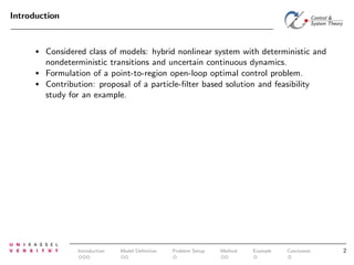
Control methods for Stochastic Hybrid Models in the literature (as far as
relevant for this paper):
Method specification
optimal
control
[1]
particle
filter
chance
constraints
nonlinear
dynamics
-
-
[2]
Model specification
uncertain
dynamics
-
-
[3]
-
[4]
[6]
[1]:
[2]:
[3]:
[4]:
[5]:
[6]:
-
-
-
-
[5]
stochastic deterministic
events
events
-
-
-
-
-
-
-
-
-
-
Bemporad et. al.: Model-Predictive Control of Discrete Hybrid Stochastic Automata, 2011,
Blackmore et. al.: Optimal Robust Predictive Control of Nonlinear Systems under Probabilistic Uncertainty using Particles, 2007,
Adamek et. al.: Stochastic Optimal Control for Hybrid Systems with Uncertain Dynamics, 2008,
Ding et. al.: Increasing Efficiency of Optimization-based Path Planning for Robotic Manipulators, 2011,
Li et. al.: Risk-Sensitive Cubature Filtering for Jump Markov Nonlinear Systems and Its Application to Land Vehicle Positioning, 2011,
Vitus et. al.: Closed-Loop Belief Space Planning for Linear, Gaussian Systems, 2011
Introduction
Model Definition
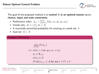
Problem Setup
Method
Example
Conclusion
4](https://image.slidesharecdn.com/adhs12-140110020412-phpapp02/85/Control-of-Uncertain-Hybrid-Nonlinear-Systems-Using-Particle-Filters-6-320.jpg)
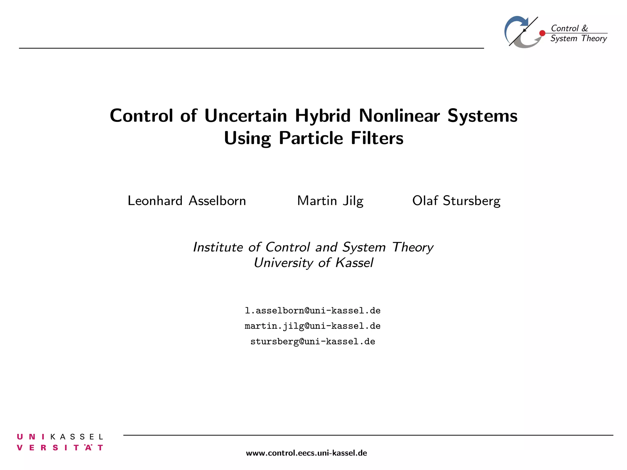
![Considered Class of Model
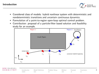
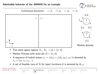
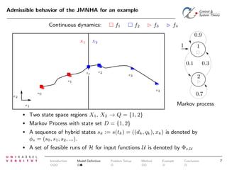
The “Jump Markov Nonlinear Hybrid Automaton (JMNHA)”:
• No resets in the continuous state variable for autonomous transitions
based on a state space partition
•
Spontaneous transitions according to a Markov Process.
•
Uncertain nonlinear dynamics: deterministic behavior for t ∈]tk , tk+1 [,
stochastic pertubation at tk .
→ Model simplification by evaluating the nondeterministic events in discrete
time.
Introduction
Model Definition
Problem Setup
Method
Example
Conclusion
5](https://image.slidesharecdn.com/adhs12-140110020412-phpapp02/85/Control-of-Uncertain-Hybrid-Nonlinear-Systems-Using-Particle-Filters-7-320.jpg)
![Considered Class of Model
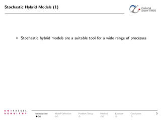
The “Jump Markov Nonlinear Hybrid Automaton (JMNHA)”:
• No resets in the continuous state variable for autonomous transitions
based on a state space partition
•
Spontaneous transitions according to a Markov Process.
•
Uncertain nonlinear dynamics: deterministic behavior for t ∈]tk , tk+1 [,
stochastic pertubation at tk .
PDMP
→ Model simplification by evaluating the nondeterministic events in discrete
time.
Introduction
Model Definition
Problem Setup
Method
Example
Conclusion
5](https://image.slidesharecdn.com/adhs12-140110020412-phpapp02/85/Control-of-Uncertain-Hybrid-Nonlinear-Systems-Using-Particle-Filters-8-320.jpg)
![Considered Class of Model
The “Jump Markov Nonlinear Hybrid Automaton (JMNHA)”:
• No resets in the continuous state variable for autonomous transitions
based on a state space partition
•
Spontaneous transitions according to a Markov Process.
•
Uncertain nonlinear dynamics: deterministic behavior for t ∈]tk , tk+1 [,
stochastic pertubation at tk .
PDMP
→ Model simplification by evaluating the nondeterministic events in discrete
time.
Introduction
Model Definition
Problem Setup
Method
Example
Conclusion
5](https://image.slidesharecdn.com/adhs12-140110020412-phpapp02/85/Control-of-Uncertain-Hybrid-Nonlinear-Systems-Using-Particle-Filters-9-320.jpg)
![Considered Class of Model
The “Jump Markov Nonlinear Hybrid Automaton (JMNHA)”:
• No resets in the continuous state variable for autonomous transitions
based on a state space partition
•
Spontaneous transitions according to a Markov Process.
•
Uncertain nonlinear dynamics: deterministic behavior for t ∈]tk , tk+1 [,
stochastic pertubation at tk .
PDMP
→ Model simplification by evaluating the nondeterministic events in discrete
time.
Introduction
Model Definition
Problem Setup
Method
Example
Conclusion
5](https://image.slidesharecdn.com/adhs12-140110020412-phpapp02/85/Control-of-Uncertain-Hybrid-Nonlinear-Systems-Using-Particle-Filters-10-320.jpg)
![Considered Class of Model
The “Jump Markov Nonlinear Hybrid Automaton (JMNHA)”:
• No resets in the continuous state variable for autonomous transitions
based on a state space partition
•
Spontaneous transitions according to a Markov Process.
•
Uncertain nonlinear dynamics: deterministic behavior for t ∈]tk , tk+1 [,
stochastic pertubation at tk .
PDMP
JMNHA
→ Model simplification by evaluating the nondeterministic events in discrete
time.
Introduction
Model Definition
Problem Setup
Method
Example
Conclusion
5](https://image.slidesharecdn.com/adhs12-140110020412-phpapp02/85/Control-of-Uncertain-Hybrid-Nonlinear-Systems-Using-Particle-Filters-11-320.jpg)
![Considered Class of Model
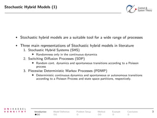
The “Jump Markov Nonlinear Hybrid Automaton (JMNHA)”:
• No resets in the continuous state variable for autonomous transitions
based on a state space partition
•
Spontaneous transitions according to a Markov Process.
•
Uncertain nonlinear dynamics: deterministic behavior for t ∈]tk , tk+1 [,
stochastic pertubation at tk .
xk+1
PDMP
xk
xk+1 = xk +
tk+1
t
f (τ )dτ + νk
k
JMNHA
→ Model simplification by evaluating the nondeterministic events in discrete
time.
Introduction
Model Definition
Problem Setup
Method
Example
Conclusion
5](https://image.slidesharecdn.com/adhs12-140110020412-phpapp02/85/Control-of-Uncertain-Hybrid-Nonlinear-Systems-Using-Particle-Filters-12-320.jpg)
![A class of Stochastic Hybrid Systems
Definition 1:
A Jump Markov Nonlinear Hybrid Automaton is defined by
H = (T, Tk , Z, X, U, U, f, ψq , ψd , ν)
with t ∈ T , tk ∈ Tk
•
nonlinear continuous dynamics x = f (x, u, d, q), x(t) ∈ X, u(t) ∈ U ,
˙
d(tk ) ∈ D, q(tk ) ∈ Q
•
hybrid state space S = X × Z, x ∈ X, z = (d, q) ∈ Z
•
update function ψq : X × X → 2Q for the state space region
•
update function ψd : D × D → [0, 1]nd for the Markov process
•
uncertainty ν in the continuous state variable x, xk+1 = xk+1 + νk+1
ˇ
Introduction
Model Definition
Problem Setup
Method
Example
Conclusion
6](https://image.slidesharecdn.com/adhs12-140110020412-phpapp02/85/Control-of-Uncertain-Hybrid-Nonlinear-Systems-Using-Particle-Filters-13-320.jpg)
![Approximation by Particle Filters
The main properties of a Particle Filter
1
1
[2]: L. Blackmore, B. C. Williams: Optimal Robust Predictive Control of Nonlinear Systems
under Probabilistic Uncertainty using Particles, 2007
Introduction
Model Definition
Problem Setup
Method
Example
Conclusion
9](https://image.slidesharecdn.com/adhs12-140110020412-phpapp02/85/Control-of-Uncertain-Hybrid-Nonlinear-Systems-Using-Particle-Filters-22-320.jpg)
![Approximation by Particle Filters
The main properties of a Particle Filter
1
•
A particle represents a sample of a random variable Ξ drawn from a given
probability distribution: ξ (1) , . . . , ξ (N)
•
The expected value can be approximated by the sample mean:
N
1
(i)
ˆ
E(Ξ) = N
i=1 ξ
•
Each particle represents a deterministic realization of the JMNHA over a finite
horizon.
1
[2]: L. Blackmore, B. C. Williams: Optimal Robust Predictive Control of Nonlinear Systems
under Probabilistic Uncertainty using Particles, 2007
Introduction
Model Definition
Problem Setup
Method
Example
Conclusion
9](https://image.slidesharecdn.com/adhs12-140110020412-phpapp02/85/Control-of-Uncertain-Hybrid-Nonlinear-Systems-Using-Particle-Filters-23-320.jpg)
![Approximation by Particle Filters
The main properties of a Particle Filter
1
•
A particle represents a sample of a random variable Ξ drawn from a given
probability distribution: ξ (1) , . . . , ξ (N)
•
The expected value can be approximated by the sample mean:
N
1
(i)
ˆ
E(Ξ) = N
i=1 ξ
•
Each particle represents a deterministic realization of the JMNHA over a finite
horizon.
The particles are used to transform a stochastic optimization problem into
a deterministic variant.
1
[2]: L. Blackmore, B. C. Williams: Optimal Robust Predictive Control of Nonlinear Systems
under Probabilistic Uncertainty using Particles, 2007
Introduction
Model Definition
Problem Setup
Method
Example
Conclusion
9](https://image.slidesharecdn.com/adhs12-140110020412-phpapp02/85/Control-of-Uncertain-Hybrid-Nonlinear-Systems-Using-Particle-Filters-24-320.jpg)
![Approximation by Particle Filters
The main properties of a Particle Filter
1
•
A particle represents a sample of a random variable Ξ drawn from a given
probability distribution: ξ (1) , . . . , ξ (N)
•
The expected value can be approximated by the sample mean:
N
1
(i)
ˆ
E(Ξ) = N
i=1 ξ
•
Each particle represents a deterministic realization of the JMNHA over a finite
horizon.
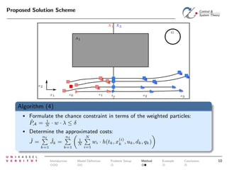
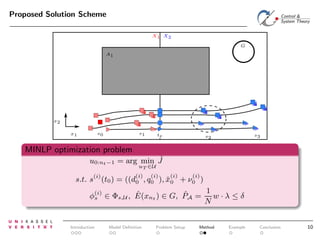
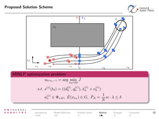
The particles are used to transform a stochastic optimization problem into
a deterministic variant.
The setup of a chance constraint
(i)
•
Indicator function 1A (x1:nt ) denotes if the i-th trajectory is in A at any time.
•
Binary vector λ ∈ {0, 1}N×1 is used for a mixed integer formulation:
1
ˆ
PA = N · w · λ ≤ δ with weighting vector w.
1
[2]: L. Blackmore, B. C. Williams: Optimal Robust Predictive Control of Nonlinear Systems
under Probabilistic Uncertainty using Particles, 2007
Introduction
Model Definition
Problem Setup
Method
Example
Conclusion
9](https://image.slidesharecdn.com/adhs12-140110020412-phpapp02/85/Control-of-Uncertain-Hybrid-Nonlinear-Systems-Using-Particle-Filters-25-320.jpg)
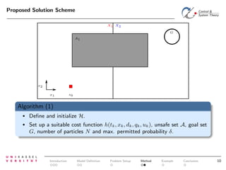
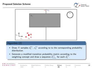
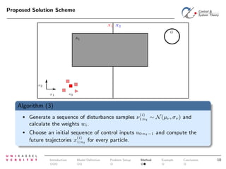
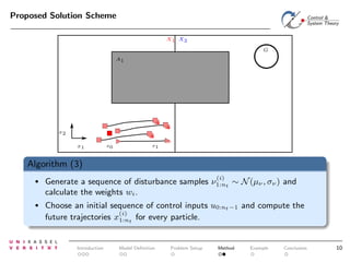
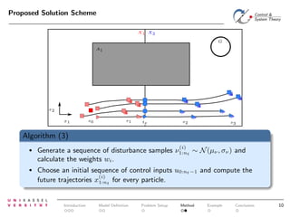

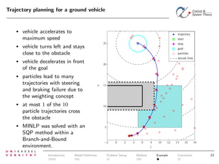

The document discusses controlling uncertain hybrid nonlinear systems using a particle filter-based approach for robust optimal control. It outlines the formulation of a point-to-region open-loop control problem and describes the 'jump markov nonlinear hybrid automaton' model that incorporates both deterministic and stochastic elements. The proposed method aims to minimize the probability of entering unsafe states while achieving performance goals under uncertainties.


![Av 738- Adaptive Filtering - Wiener Filters[wk 3]](https://cdn.slidesharecdn.com/ss_thumbnails/av-738-aft-spr18-lecture03-optimumfilters-weinerwk3-180215235757-thumbnail.jpg?width=640&height=640&fit=bounds)

![Sensor Fusion Study - Ch15. The Particle Filter [Seoyeon Stella Yang]](https://cdn.slidesharecdn.com/ss_thumbnails/particlefilter-200815094542-thumbnail.jpg?width=640&height=640&fit=bounds)