This chapter discusses the principle of microscopic reversibility and its implications. It can be summarized as follows: 1) The principle of microscopic reversibility states that the probability of a molecular process occurring is equal to the probability of the reverse process at equilibrium. 2) This leads to the rule of detailed balances and Onsager's reciprocity relations, which relate the linear response of a system to external perturbations to its intrinsic fluctuation properties. 3) The reciprocity relations require that the Onsager coefficients relating fluxes to forces be symmetric. Various formulations of the fluctuation-dissipation theorem are also derived from microscopic reversibility.

1. Chapter 2
Microscopic Reversibility
The Principle of Microscopic Reversibility was formulated by Richard Tolman [14]
who stated that, at equilibrium, “any molecular process and the reverse of that pro-
cess will be taking place on the average at the same rate”. Applying this concept
to macroscopic systems at local equilibrium leads to the rule of detailed balances
(Sect. 2.2) and then, assuming linear relations between thermodynamic forces and
fluxes, to the formulation of the celebrated reciprocity relations (Sect. 2.3) derived
by Lars Onsager in 1931, and the fluctuation-dissipation theorem, (Sect. 2.4) proved
by Herbert Callen and Theodore Welton in 1951. In this chapter, this vast subject
matter is treated with a critical attitude, stressing all the hypotheses and their limi-
tations.
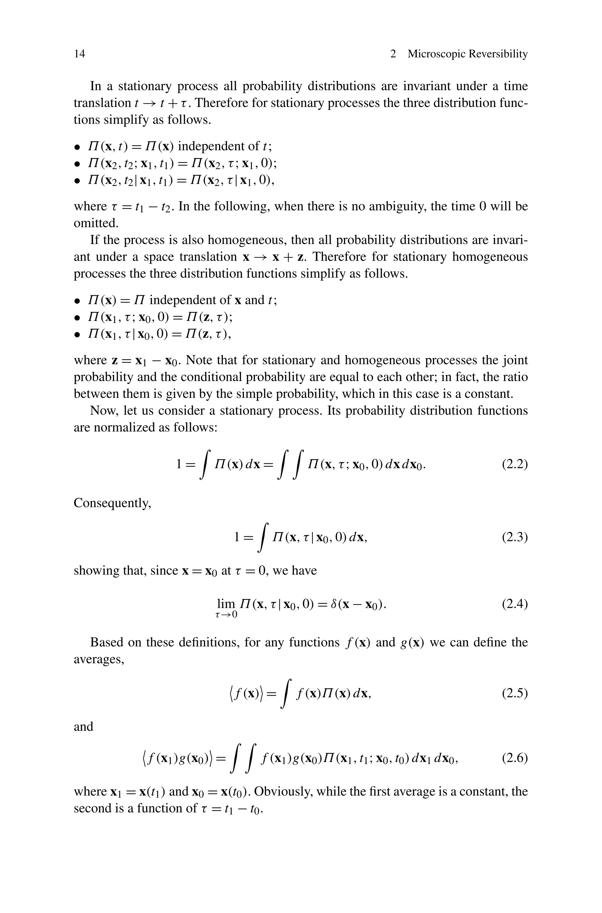
2.1 Probability Distributions
Define:
• The simple probability Π(x,t) that the random variable x(t) has a certain value
x at time t.1
• The joint probability Π(x2,t2;x1,t1) that the random variable x(t) has a certain
value x2 = x(t2) at time t2 and, also, that it has another value x1 = x(t1) at time t1.
• The conditional probability Π(x2,t2|x1,t1) that a random variable x has a certain
value x2 = x(t2) at time t2, provided that at another (i.e. previous) time t1 it has a
value x1 = x(t1).
By definition, when t2 > t1,
Π(x2,t2;x1,t1) = Π(x2,t2|x1,t1)Π(x1,t1). (2.1)
1Here and in the following, we use the same notation, x, to indicate both the random variable and
the value that it can assume. Whenever this might be confusing, different symbols will be used.
R. Mauri, Non-Equilibrium Thermodynamics in Multiphase Flows,
Soft and Biological Matter, DOI 10.1007/978-94-007-5461-4_2,
© Springer Science+Business Media Dordrecht 2013
13

2. 14 2 Microscopic Reversibility
In a stationary process all probability distributions are invariant under a time
translation t → t + τ. Therefore for stationary processes the three distribution func-
tions simplify as follows.
• Π(x,t) = Π(x) independent of t;
• Π(x2,t2;x1,t1) = Π(x2,τ;x1,0);
• Π(x2,t2|x1,t1) = Π(x2,τ|x1,0),
where τ = t1 − t2. In the following, when there is no ambiguity, the time 0 will be
omitted.
If the process is also homogeneous, then all probability distributions are invari-
ant under a space translation x → x + z. Therefore for stationary homogeneous
processes the three distribution functions simplify as follows.
• Π(x) = Π independent of x and t;
• Π(x1,τ;x0,0) = Π(z,τ);
• Π(x1,τ|x0,0) = Π(z,τ),
where z = x1 − x0. Note that for stationary and homogeneous processes the joint
probability and the conditional probability are equal to each other; in fact, the ratio
between them is given by the simple probability, which in this case is a constant.
Now, let us consider a stationary process. Its probability distribution functions
are normalized as follows:
1 = Π(x)dx = Π(x,τ;x0,0)dxdx0. (2.2)
Consequently,
1 = Π(x,τ|x0,0)dx, (2.3)
showing that, since x = x0 at τ = 0, we have
lim
τ→0
Π(x,τ|x0,0) = δ(x − x0). (2.4)
Based on these definitions, for any functions f (x) and g(x) we can define the
averages,
f (x) = f (x)Π(x)dx, (2.5)
and
f (x1)g(x0) = f (x1)g(x0)Π(x1,t1;x0,t0)dx1 dx0, (2.6)
where x1 = x(t1) and x0 = x(t0). Obviously, while the first average is a constant, the
second is a function of τ = t1 − t0.

3. 2.2 Microscopic Reversibility 15
We can also define the conditional average of any functions f (x) of the random
variable x(t) as the mean value of f (x) at time τ, assuming that x(0) = x0, i.e.,
f (x)
x0
τ
= f (x)Π[x,τ|x0,0]dx. (2.7)
This conditional average depends on τ and on x0.
Now, substituting (2.1) into (2.6), we obtain the following equality,
f (x)g(x0) = f (x)g(x0)Π(x,τ|x0,0)Π(x0)dxdx0, (2.8)
that is:
f (x)g(x0) = f (x)
x0
τ
g(x0) . (2.9)
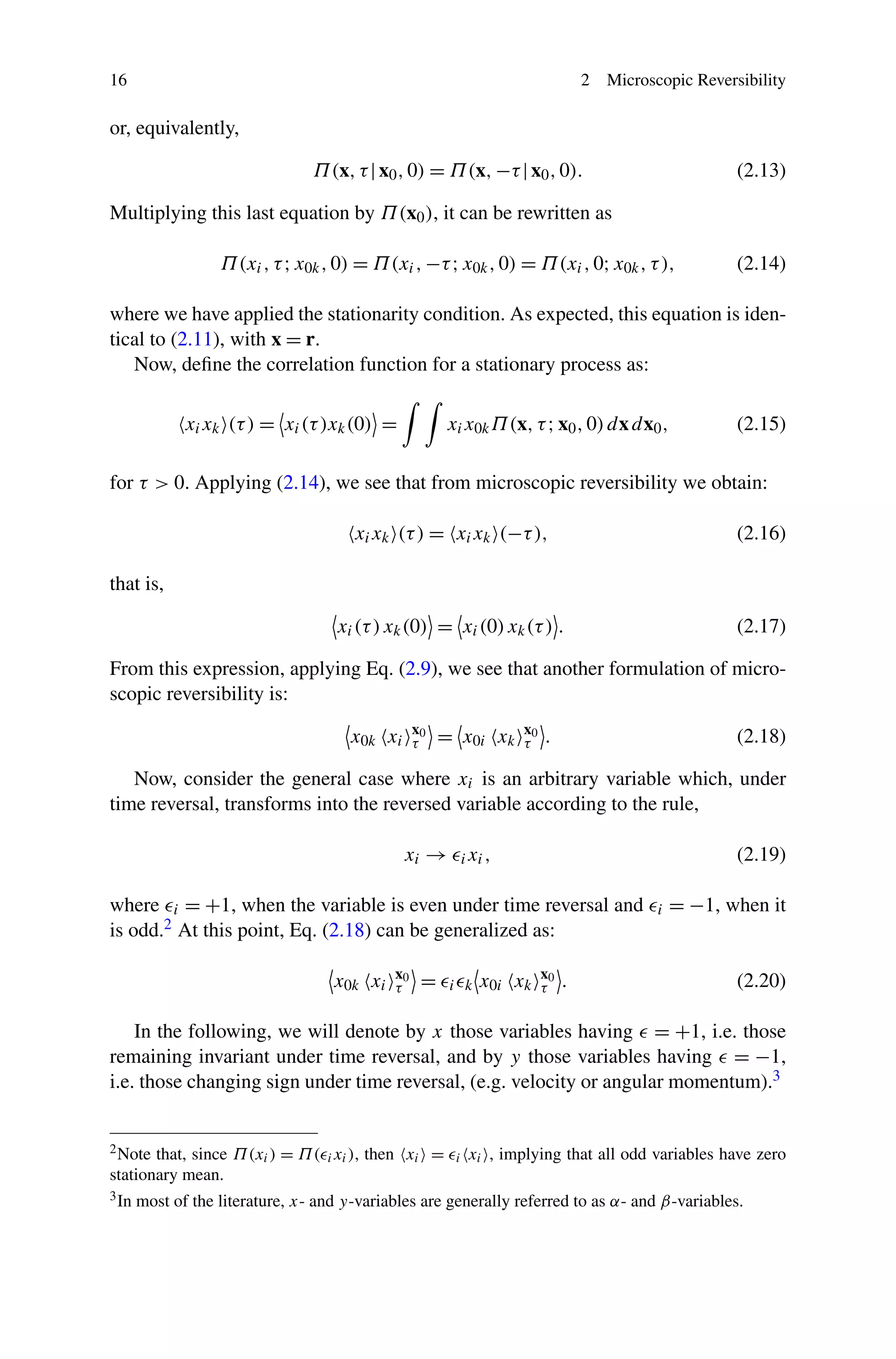
2.2 Microscopic Reversibility
For a classical N-body system with conservative forces, microscopic reversibility is
a consequence of the invariance of the equations of motion under time reversal and
simply means that for every microscopic motion reversing all particle velocities also
yield a solution. More precisely, the equations of motion of an N particle system are
invariant under the transformation
τ → −τ; r → r; v → −v, (2.10)
where r ≡ rN and v ≡ vN are the positions and the velocities of the N particles.
This leads to the so-called principle of detailed balance, stating that in a stationary
situation each possible transition (ˆr, ˆv) → (r,v) balances with the time reversed
transition (r,−v) → (ˆr,−ˆv), so that,
Π r(τ),v(τ); ˆr(0), ˆv(0) = Π ˆr(τ),−ˆv(τ); r(0),−v(0) . (2.11)
As we saw in Sect. 1.1, this same condition can be applied when we deal with
thermodynamic, coarse grained variables at local equilibrium, i.e. when τ ≤ τf luct ,
where τf luct is the typical fluctuation time. In fact, for such very short times, forward
motion is indistinguishable from backward motion, as they both are indistinguish-
able from fluctuations.
First, let us consider variables xi(t) that are invariant under time reversal, e.g.
they are even functions of the particle velocities. In this case, another, perhaps more
intuitive, way to write the principle of detailed balance is to assume that the condi-
tional mean values of a variable at times τ and −τ are equal to each other, which
means,
x x0
τ = x
x0
−τ (2.12)

4. 16 2 Microscopic Reversibility
or, equivalently,
Π(x,τ|x0,0) = Π(x,−τ|x0,0). (2.13)
Multiplying this last equation by Π(x0), it can be rewritten as
Π(xi,τ;x0k,0) = Π(xi,−τ;x0k,0) = Π(xi,0;x0k,τ), (2.14)
where we have applied the stationarity condition. As expected, this equation is iden-
tical to (2.11), with x = r.
Now, define the correlation function for a stationary process as:
xixk (τ) = xi(τ)xk(0) = xix0kΠ(x,τ;x0,0)dxdx0, (2.15)
for τ > 0. Applying (2.14), we see that from microscopic reversibility we obtain:
xixk (τ) = xixk (−τ), (2.16)
that is,
xi(τ)xk(0) = xi(0)xk(τ) . (2.17)
From this expression, applying Eq. (2.9), we see that another formulation of micro-
scopic reversibility is:
x0k xi
x0
τ = x0i xk
x0
τ . (2.18)
Now, consider the general case where xi is an arbitrary variable which, under
time reversal, transforms into the reversed variable according to the rule,
xi → ixi, (2.19)
where i = +1, when the variable is even under time reversal and i = −1, when it
is odd.2 At this point, Eq. (2.18) can be generalized as:
x0k xi
x0
τ = i k x0i xk
x0
τ . (2.20)
In the following, we will denote by x those variables having = +1, i.e. those
remaining invariant under time reversal, and by y those variables having = −1,
i.e. those changing sign under time reversal, (e.g. velocity or angular momentum).3
2Note that, since Π(xi) = Π( ixi), then xi = i xi , implying that all odd variables have zero
stationary mean.
3In most of the literature, x- and y-variables are generally referred to as α- and β-variables.

5. 2.3 Onsager’s Reciprocity Relations 17
2.3 Onsager’s Reciprocity Relations
Assume the following linear phenomenological relations: (i.e. neglecting fluctua-
tions)
˙xi =
n
j=1
Lij Xj , (2.21)
where the dot denotes time derivative, ˙x are referred to as thermodynamic fluxes,
while X are the generalized forces defined in (1.16). That means that this equation
holds when we apply it to its conditional averages,
˙xi
x0
τ =
n
j=1
Lij Xj
x0
τ . (2.22)
The coefficients Lij are generally referred to as Onsager’s, or phenomenological,
coefficients. Now take the time derivative of Eq. (2.18), considering that x0 is con-
stant:
n
j=1
Lij x0k Xj
x0
τ =
n
j=1
Lkj x0i Xj
x0
τ . (2.23)
Considering that Xj
x0
τ=0 = X0j and x0iX0j = −δij , we obtain:
Lik = Lki. (2.24)
These are the celebrated reciprocity relations, derived by Lars Onsager [12, 13] in
1931.
In the presence of a magnetic field B or when the system rotates with angular ve-
locity , the operation of time reversal implies, besides the transformation (2.10),
the reversal of B and as well. Therefore, the Onsager reciprocity relations be-
come:
Lik(B, ) = Lki(−B,− ). (2.25)
In the following, we will assume that B = 0 and = 0; however, we should keep
in mind that in the presence of magnetic fields or overall rotations, the Onsager
relations can be applied only when B and are reversed.
A clever way to express the Onsager coefficients Lij can be obtained by multi-
plying Eq. (2.22) by x0k and averaging:
x0k ˙xi
x0
τ =
n
j=1
Lij x0k Xj
x0
τ . (2.26)
Now take τ = 0 and apply Eq. (2.9) to obtain:
Lik = − ˙xixk
sym
0 , (2.27)

6. 18 2 Microscopic Reversibility
where the superscript “sym” indicates the symmetric part of a tensor, i.e. A
sym
ij =
1
2 (Aij + Aji). This is one of the many forms of the fluctuation-dissipation theorem,
which states that the linear response of a given system to an external perturbation
is expressed in terms of fluctuation properties of the system in thermal equilibrium.
Although it was formulated by Nyquist in 1928 to determine the voltage fluctuations
in electrical impedances [11], the fluctuation-dissipation theorem was first proven
in its general form by Callen and Welton [3] in 1951.
In (2.27), ˙x is the velocity of the random variable as it relaxes to equilib-
rium. Therefore, considering that x tends to 0 for long times, we see that x(0) =
−
∞
0 ˙x(t)dt and therefore the fluctuation-dissipation theorem can also be formu-
lated through the following Green-Kubo relation:4
Lik =
∞
0
˙xi(0)˙xk(t)
sym
dt, (2.28)
showing that the Onsager coefficients can be expressed as the time integral of the
correlation function between the velocities of the random variables at two different
times.
Now, consider the opposite process, where the random variable evolves out of its
equilibrium position x = 0. Therefore, applying again Eq. (2.27), but with negative
times, we obtain:
Lik =
1
2
d
dt
xixk
sym
0 , (2.29)
showing that the Onsager coefficients can be expressed as the temporal growth of the
mean square displacements of the system variables from their equilibrium values.
These results are easily extended to the case where we have both x and y-
variables, i.e. even and odd variables under time reversal. In this case, the phe-
nomenological equations (2.21) can be generalized as:
˙xi =
n
j=1
L
(xx)
ij Xj +
n
j=1
L
(xy)
ij Yj , (2.30)
˙yi =
n
j=1
L
(yx)
ij Xj +
n
j=1
L
(yy)
ij Yj , (2.31)
where
Xi =
1
k
∂ S
∂xi
; Yi =
1
k
∂ S
∂yi
(2.32)
are the thermodynamic forces associated with the x and y-variables, respectively.
With the help of these quantities, the reciprocity relations (2.24) were generalized
4The Green-Kubo relation is also called the fluctuation-dissipation theorem of the second kind.
See [7, 8].

7. 2.3 Onsager’s Reciprocity Relations 19
by Casimir in 1945 as [4]:
L
(xx)
ij = L
(xx)
ji ; L
(xy)
ij = −L
(yx)
ji ; L
(yy)
ij = L
(yy)
ji . (2.33)
Substituting (2.30), (2.31) and (2.33) into the generalized form (1.26) of the en-
tropy production term,
1
k
dS
dt
=
n
i=1
˙xiXi +
n
i=1
˙yiYi, (2.34)
we obtain:
1
k
d
dt
S =
n
i=1
n
j=1
L(xx)
ij XiXj +
n
i=1
n
j=1
L
(yy)
ij YiYj . (2.35)
This shows that neither the antisymmetric parts of the Onsager coefficients L(xx)
and L(yy), nor the coupling terms between x and y-variables, L(xy) and L(yx), give
any contribution to the entropy production rate.
It should be stressed that, when we apply the Onsager-Casimir reciprocity rela-
tions, we must make sure that the n variables (and therefore their time derivatives,
or fluxes, as well) are independent from each other, and similarly for the thermody-
namic forces.5
Comment 2.1 In the course of deriving the reciprocity relations, we have assumed
that the same equations (2.21) govern both the macroscopic evolution of the system
and the relaxation of its spontaneous deviations from equilibrium. This condition is
often referred to as Onsager’s postulate and is the basis of the Langevin equation
(see Chap. 3).6 The fluctuation-dissipation theorem, Eqs. (2.29) and (2.41), can be
seen as a natural consequence of this postulate.
Comment 2.2 The simplest way to see the meaning of the fluctuation-dissipation
theorem is to consider the free diffusion of Brownian particles (see Sect. 3.1). First,
consider a homogeneous system, follow a single particle as it moves randomly
around7 and define a coefficient of self-diffusion as (one half of) the time deriva-
tive of its mean square displacement. Then, take the system out of equilibrium, and
define the gradient diffusivity as the ratio between the material flux resulting from
an imposed concentration gradient and the concentration gradient itself. As shown
by Einstein in his Ph.D. thesis on Brownian motion [6], when the problem is lin-
ear (i.e. when particle-particle interactions are neglected), these two diffusivities are
5As shown in [10], when fluxes and forces are not independent, but still linearly related to one
another, there is a certain arbitrariness in the choice of the independent variables, so that at the end
the phenomenological coefficients can be chosen to satisfy the Onsager relations.
6Onsager stated that “the average regression of fluctuations will obey the same laws as the corre-
sponding macroscopic irreversible process”. See discussions in [9, 15].
7This process is sometimes called Knudsen effusion.

8. 20 2 Microscopic Reversibility
equal to each other, thus establishing perhaps the simplest example of fluctuation-
dissipation theorem. Although we take this result for granted, it is far from obvious,
as it states the equality between two very different quantities: on one hand, the fluc-
tuations of a system when it is macroscopically at equilibrium; on the other hand,
its dissipative properties as it approaches equilibrium.
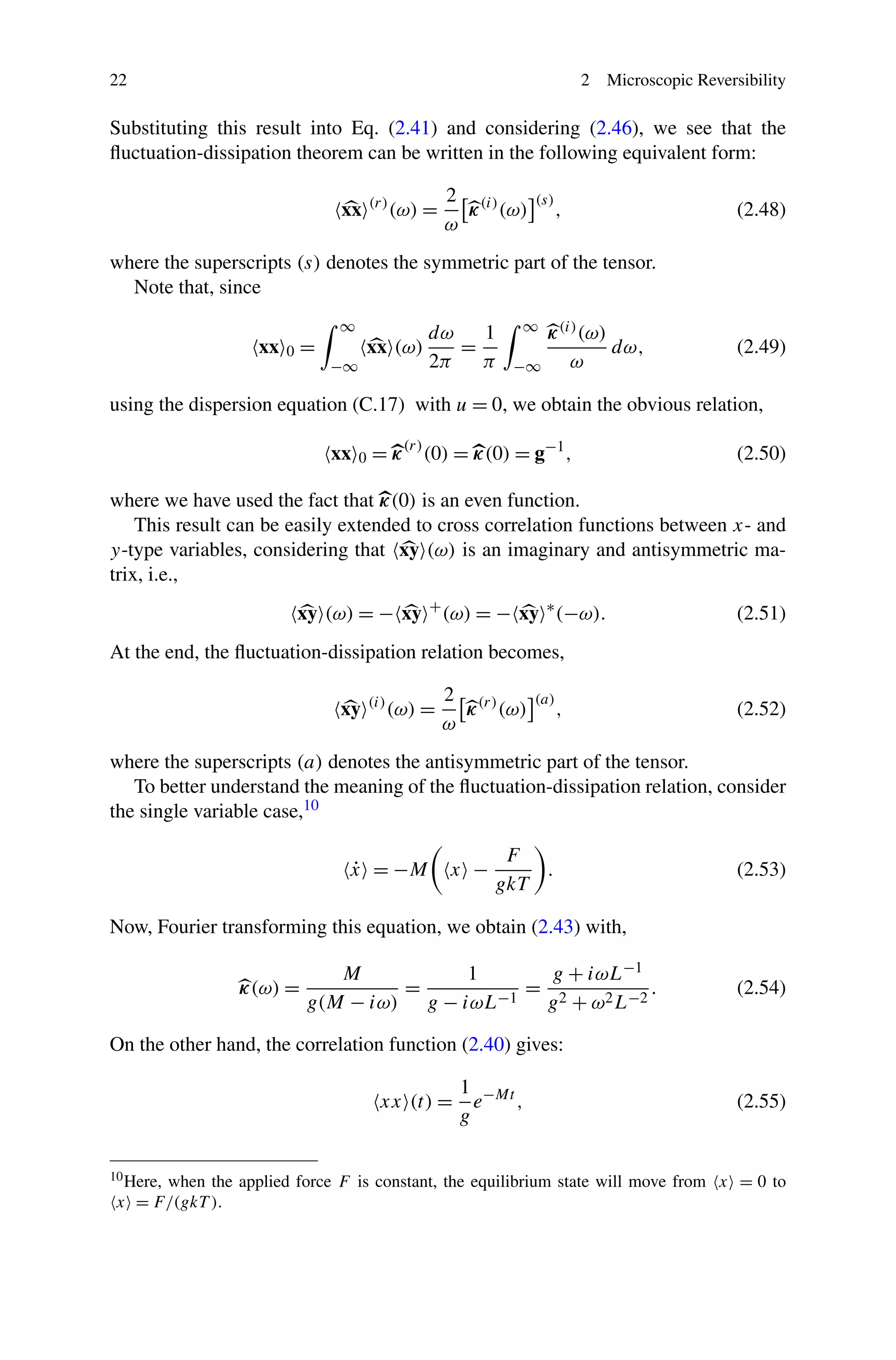
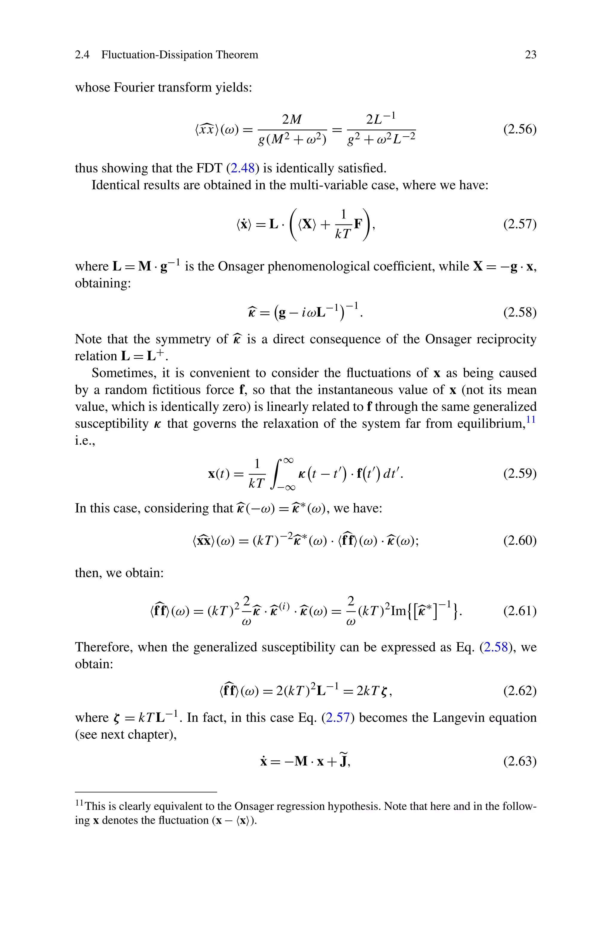
2.4 Fluctuation-Dissipation Theorem
As we saw in the previous section, the fluctuation-dissipation theorem (FDT) con-
nects the linear response relaxation of a system to its statistical fluctuation properties
at equilibrium and it relies on Onsager’s postulate that the response of a system in
thermodynamic equilibrium to a small applied force is the same as its response to a
spontaneous fluctuation.
First, let us derive the FDT in a very simple and intuitive way, following the
original formulation by Callen and Greene [1, 2]. Assume that a constant thermo-
dynamic force X0 = −F0/kT is applied to the system for an infinite time t < 0 and
then it is suddenly turned off at t = 0. Therefore, at t = 0 the system will have a
non-zero position of stable equilibrium, x0, such that
F0 = ∇xWmin = kT g · x0, (2.36)
where Wmin = 1
2 kT x0 · g · x0 = F0 · x0 is the minimum work that the constant force,
F0, has to exert to displace the system to position x0.
Now, in the absence of any external force, i.e. when t > 0, the mean value of the
x-variable relaxes in time following Eq. (2.22), with,
˙x x0 (t) = −M · x x0 (t); i.e., x x0 (t) = exp(−Mt) · x0, (2.37)
where M = L · g is a constant phenomenological relaxation coefficient. Therefore,
substituting (2.36) into (2.37) we obtain:
x x0 (t) = χ(t) ·
F0
kT
, (2.38)
where
χ(t) = exp(−Mt) · g−1
(2.39)
is a time dependent relaxation coefficient.
On the other hand, the function χ is related to the correlation function at equilib-
rium, xx . In fact, from the definition (2.15), substituting (2.37) we see that:
xx (t) = x
x0
t x0 = exp(−Mt) · x0x0 = exp(−Mt) · g−1
. (2.40)

9. 2.4 Fluctuation-Dissipation Theorem 21
Comparing the last two equations, we conclude:
xx (t) = χ(t). (2.41)
This relation represents the fluctuation-dissipation theorem.8
Note that, when t = 0, the relation (2.41) is identically satisfied, since xx (0) =
g−1, while χ(0) = g−1.
The fluctuation-dissipation theorem can also be determined assuming a general,
time-dependent driving force, F(t). In this case, due to the linearity of the process,
we can write:
x(t) =
1
kT
∞
−∞
κ t − t · F t dt , (2.42)
where κ(t) is the generalized susceptibility, with κ(t) = 0 for t < 0. Denoting by
x(ω), κ(ω) and X(ω), the Fourier transforms (C.1) of x(t) , κ(t) and X(t), respec-
tively, we have:
x(ω) =
1
kT
κ(ω) · F(ω). (2.43)
In general, κ(ω) is a complex function, with κ = κ(r) +iκ(i), where the superscripts
(r) and (i) indicate the real and imaginary part. Since κ(t) is real, we have:
κ(−ω) = κ∗
(ω), (2.44)
where the asterisk indicates complex conjugate, showing that κ(r) is an even func-
tion, while κ(i) is an odd function, i.e.,
κ(r)
(−ω) = κ(r)
(ω); κ(i)
(−ω) = −κ(i)
(ω). (2.45)
Analogous relations exists regarding the correlation function xx (t). In fact,
considering the microscopic reversibility (2.16) and the reality condition, we ob-
tain:
xx (ω) = xx +
(ω) = xx ∗
(−ω), (2.46)
i.e. the Fourier transform of the correlation function is a real and symmetric matrix.
As shown in Appendix C, using the causality principle, i.e. imposing that κ(t) =
0 for t < 0, we see that the generalized susceptibility is subjected to the Kramers-
Kronig relation (C.17), so that κ(t) can be related to χ(t) as [cf. Eq. (C.30)]9
χ(ω) =
2
iω
κ(ω). (2.47)
8The same result can be obtained assuming that the constant thermodynamic force X0 is suddenly
turned on at t = 0, so that for long times the system will have a non-zero position of stable equi-
librium, xF = −g−1 · X0. In that case, redefining the random variable x as xF − x, we find again
Eq. (2.41).
9This is a somewhat simplified analysis. For more details, see [5].

10. 22 2 Microscopic Reversibility
Substituting this result into Eq. (2.41) and considering (2.46), we see that the
fluctuation-dissipation theorem can be written in the following equivalent form:
xx (r)
(ω) =
2
ω
κ(i)
(ω)
(s)
, (2.48)
where the superscripts (s) denotes the symmetric part of the tensor.
Note that, since
xx 0 =
∞
−∞
xx (ω)
dω
2π
=
1
π
∞
−∞
κ(i)(ω)
ω
dω, (2.49)
using the dispersion equation (C.17) with u = 0, we obtain the obvious relation,
xx 0 = κ(r)
(0) = κ(0) = g−1
, (2.50)
where we have used the fact that κ(0) is an even function.
This result can be easily extended to cross correlation functions between x- and
y-type variables, considering that xy (ω) is an imaginary and antisymmetric ma-
trix, i.e.,
xy (ω) = − xy +
(ω) = − xy ∗
(−ω). (2.51)
At the end, the fluctuation-dissipation relation becomes,
xy (i)
(ω) =
2
ω
κ(r)
(ω)
(a)
, (2.52)
where the superscripts (a) denotes the antisymmetric part of the tensor.
To better understand the meaning of the fluctuation-dissipation relation, consider
the single variable case,10
˙x = −M x −
F
gkT
. (2.53)
Now, Fourier transforming this equation, we obtain (2.43) with,
κ(ω) =
M
g(M − iω)
=
1
g − iωL−1
=
g + iωL−1
g2 + ω2L−2
. (2.54)
On the other hand, the correlation function (2.40) gives:
xx (t) =
1
g
e−Mt
, (2.55)
10Here, when the applied force F is constant, the equilibrium state will move from x = 0 to
x = F/(gkT ).

11. 2.4 Fluctuation-Dissipation Theorem 23
whose Fourier transform yields:
xx (ω) =
2M
g(M2 + ω2)
=
2L−1
g2 + ω2L−2
(2.56)
thus showing that the FDT (2.48) is identically satisfied.
Identical results are obtained in the multi-variable case, where we have:
˙x = L · X +
1
kT
F , (2.57)
where L = M · g−1 is the Onsager phenomenological coefficient, while X = −g · x,
obtaining:
κ = g − iωL−1 −1
. (2.58)
Note that the symmetry of κ is a direct consequence of the Onsager reciprocity
relation L = L+.
Sometimes, it is convenient to consider the fluctuations of x as being caused
by a random fictitious force f, so that the instantaneous value of x (not its mean
value, which is identically zero) is linearly related to f through the same generalized
susceptibility κ that governs the relaxation of the system far from equilibrium,11
i.e.,
x(t) =
1
kT
∞
−∞
κ t − t · f t dt . (2.59)
In this case, considering that κ(−ω) = κ∗(ω), we have:
xx (ω) = (kT )−2
κ∗
(ω) · ff (ω) · κ(ω); (2.60)
then, we obtain:
ff (ω) = (kT )2 2
ω
κ · κ(i)
· κ(ω) =
2
ω
(kT )2
Im κ∗ −1
. (2.61)
Therefore, when the generalized susceptibility can be expressed as Eq. (2.58), we
obtain:
ff (ω) = 2(kT )2
L−1
= 2kT ζ, (2.62)
where ζ = kT L−1. In fact, in this case Eq. (2.57) becomes the Langevin equation
(see next chapter),
˙x = −M · x + J, (2.63)
11This is clearly equivalent to the Onsager regression hypothesis. Note that here and in the follow-
ing x denotes the fluctuation (x − x ).

12. 24 2 Microscopic Reversibility
where J = 1
kT L · f is the fluctuating flux, satisfying the following relation:
J(0)J(t) = 2Lδ(t), (2.64)
where δ(t) is the Dirac delta. This shows that there is no correlation between the
particle position x and the random force f (see Problem 2.2). In fact, it is this lack of
correlation that is at the foundation of the Onsager regression hypothesis, therefore
justifying the Langevin equation, as discussed in the next chapter.
2.5 Problems
Problem 2.1 Consider a small particle of arbitrary shape moving in an otherwise
quiescent Newtonian fluid. In creeping flow conditions, determine the symmetry
relations satisfied by the resistance matrix connecting velocity and angular velocity
with the force and the torque that are applied to the particle.
Problem 2.2 Consider a driven 1D oscillator of mass m at frequency ω0, with
damping force ζ ˙x, with x denoting the displacement from its equilibrium position,
x = 0. Determine the spectrum of the random force.
References
1. Callen, H.B., Greene, R.F.: Phys. Rev. 86, 702 (1952)
2. Callen, H.B., Greene, R.F.: Phys. Rev. 88, 1387 (1952)
3. Callen, H.B., Welton, T.A.: Phys. Rev. 83, 34 (1951)
4. Casimir, H.B.G.: Rev. Mod. Phys. 17, 343 (1945)
5. de Groot, S.R., Mazur, P.: Non-Equilibrium Thermodynamics. Dover, New York (1962),
Chap. VIII.4
6. Einstein, A.: Ann. Phys. (Berlin) 17, 549 (1905)
7. Green, M.S.: J. Chem. Phys. 22, 398 (1954)
8. Kubo, R.: J. Phys. Soc. Jpn. 12, 570 (1957)
9. Marconi, U.M.B., et al.: Phys. Rep. 461, 111 (2008)
10. Meixner, J.: Rheol. Acta 12, 465 (1973)
11. Nyquist, H.: Phys. Rev. 32, 110 (1928)
12. Onsager, L.: Phys. Rev. 37, 405 (1931)
13. Onsager, L.: Phys. Rev. 38, 2265 (1931)
14. Tolman, R.C.: The Principles of Statistical Mechanics, p. 163. Dover, New York (1938),
Chap. 50
15. van Kampen, N.G.: Stochastic Processes in Physics and Chemistry. North-Holland, Amster-
dam (1981), Chap. VIII.8

13. http://www.springer.com/978-94-007-5460-7