Downloaded 86 times


![17 of 60
All survey measurement observations, except RTK, should conform to the
following:
Be constrained to three or more survey project or NSRS stations, which
are located in three or more quadrants surrounding the survey project
area.
Points are connected by two or more independent baselines.
Contain valid loops with a minimum of three independent baselines.
Baselines have a fixed integer double difference solution or adhere to the
manufacturer s specifications for baseline lengths that exceed the fixed
solution criteria.
Any station pair, used as azimuth or bearing reference during
conventional survey measurements, should be included in a network, or
measured with a minimum of two independent vectors following the RTK
techniques described in Section B-I-d. Baselines between station pairs
must be measured for inclusion in network adjustment and analysis.
All stations in the survey measurements shall have two or more
independent occupations.
Single radial (spur) lines or side shots to a point are not acceptable.
Vertical Control
Based on the Federal Geographic Data Committee publication, "Geospatial
Positioning Accuracy Standards" [http://www.fgdc.gov/
standards/document/standards/accuracy], guidelines were developed by the
National Geodetic Survey (NGS) for performing GPS surveys intended to achieve
ellipsoid height network accuracies of 5 cm at the 95 percent confidence level, as
well as ellipsoid height local accuracies of 2 cm and 5 cm, also at the 95 percent
confidence level.
GPS carrier phase measurements are used to determine vector baselines in space,
where the components of the baseline are expressed in terms of Cartesian
coordinate differences. These vector baselines can be converted to distance,
azimuth, and ellipsoidal height differences (dh) relative to a defined reference
ellipsoid.](https://image.slidesharecdn.com/standardsandguidelinesforlandsurveyingusinggpsver2-151019075101-lva1-app6891/75/Standards-and-guidelines-for-land-surveying-using-gps-ver-2-1-3-17-2048.jpg)
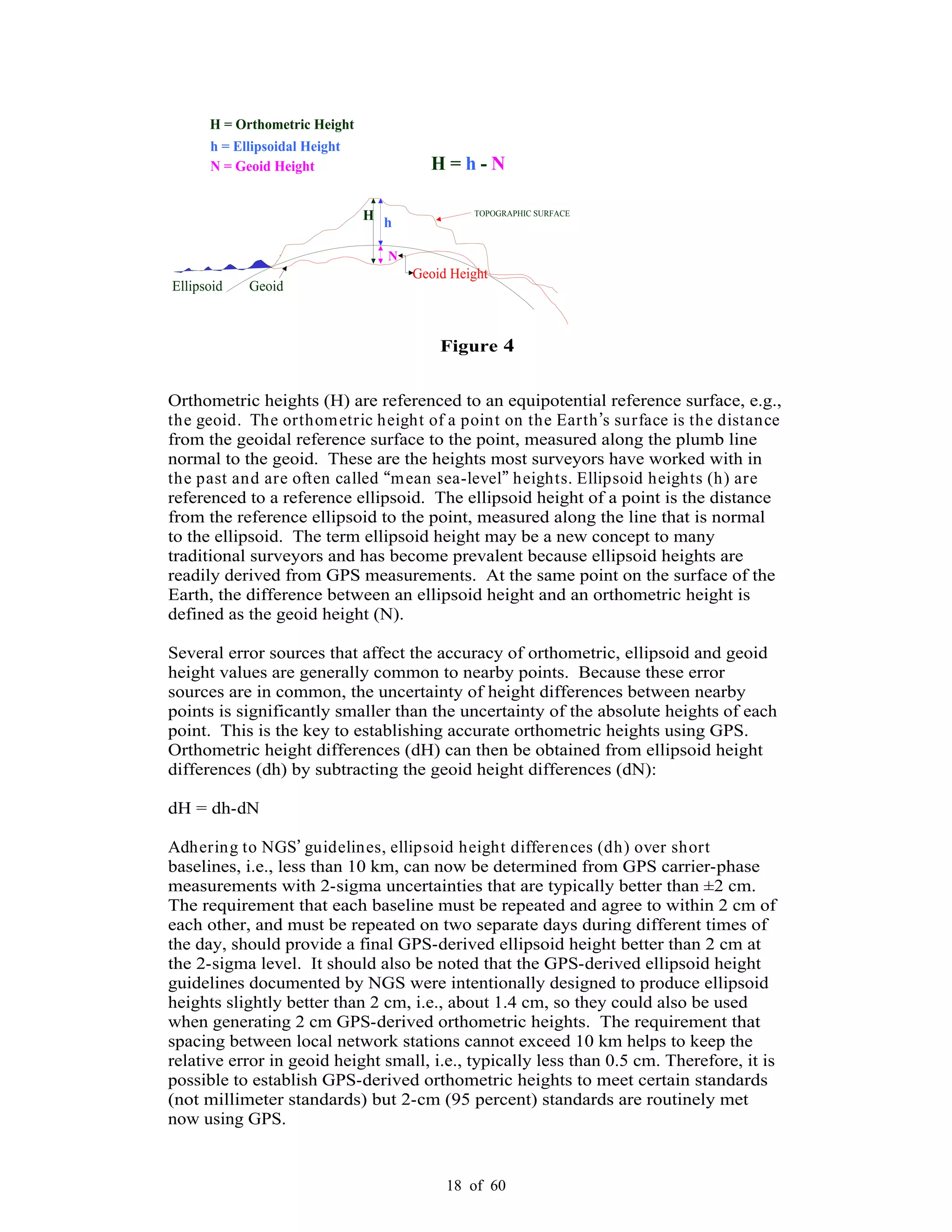
![19 of 60
There are three basic rules, four control requirements, and five procedures that
need to be adhered to for computing accurate NAVD 88 GPS-derived orthometric
heights.
Basic Rules
Rule 1: Follow NGS guidelines for establishing GPS-derived ellipsoid heights
when performing GPS surveys,
Rule 2: Use NGS latest national geoid model, e.g. GEOID03, when computing
GPS-derived orthometric heights, and
Rule 3: Use the latest National Vertical Datum, NAVD 88, height values to
control the project s adjusted heights.
Control Requirements
Requirement 1: GPS-occupy stations with valid NAVD 88 orthometric heights;
stations should be evenly distributed throughout project.
Requirement 2: For project areas less than 20 km on a side, surround project
with valid NAVD 88 bench marks, i.e., minimum number of stations is four; one
in each corner of project. [NOTE: The user may have to enlarge the project area
to occupy enough bench marks, even if the project area extends beyond the
original area of interest.]
Requirement 3: For project areas greater than 20 km on a side, keep distances
between valid GPS-occupied NAVD 88 benchmarks to less than 20 km.
Requirement 4: For projects located in mountainous regions, occupy valid
benchmarks at the base and summit of mountains, even if the distance is less
than 20 km.
Procedures
Procedure 1: Perform a 3-D minimum-constrained least squares adjustment of
the GPS survey project, i.e., constrain one latitude, one longitude, and one
orthometric height value.
Procedure 2: Using the results from the adjustment in procedure 1, detect and
remove all data outliers. [NOTE: If the user follows NGS guidelines for
establishing GPS-derived ellipsoid heights, the user will already know which
vectors may need to be rejected, and following the GPS-derived ellipsoid height
guidelines should have already re-observed those base lines.] The user should
repeat procedures 1 and 2 until all data outliers are removed.
Procedure 3: Compute the differences between the set of GPS-derived
orthometric heights from the minimum-constrained adjustment (using the](https://image.slidesharecdn.com/standardsandguidelinesforlandsurveyingusinggpsver2-151019075101-lva1-app6891/75/Standards-and-guidelines-for-land-surveying-using-gps-ver-2-1-3-19-2048.jpg)
![20 of 60
current Geoid model) from procedure 2 and the corresponding published NAVD
88 benchmarks.
Procedure 4: Using the results from procedure 3, determine which bench marks
have valid NAVD 88 height values. This is the most important step of the
process. Determining which benchmarks have valid heights is critical to
computing accurate GPS-derived orthometric heights. [NOTE: The user should
include a few extra NAVD 88 bench marks in case some are inconsistent, i.e., are
not valid NAVD 88 height values.]
Procedure 5: Using the results from procedure 4, perform a constrained
adjustment holding one latitude value, one longitude value, and all valid NAVD
88 height values fixed.
Adjustment
1. Compare repeat base lines
The procedure is very simple: subtract one ellipsoid height from the other, i.e.,
the ellipsoid height from base line A to B on day 1 minus the ellipsoid height from
base line A to B on day 2. If this difference is greater than 2 cm, one of the base
lines must be observed again. This is a very simple procedure, but also one of the
most important. Many users complain about having to repeat base lines, but
requiring an extra half-hour occupation session in the field can often save many
days of analysis in the office.
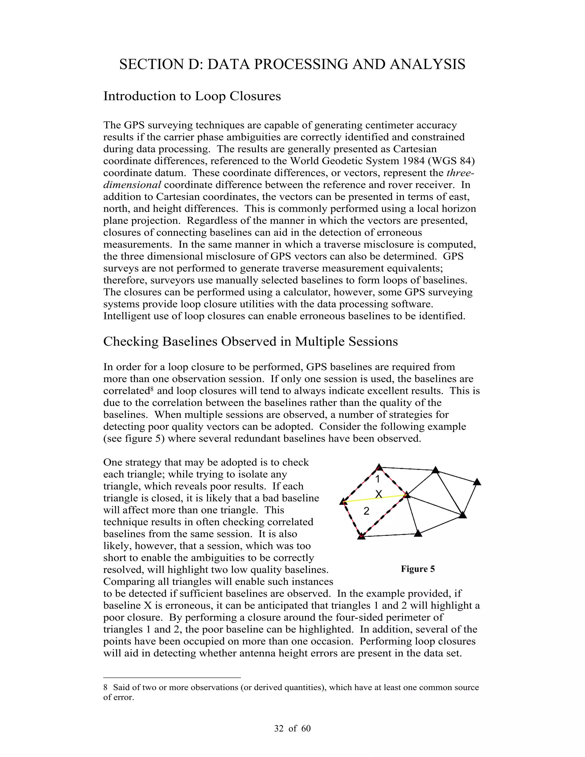
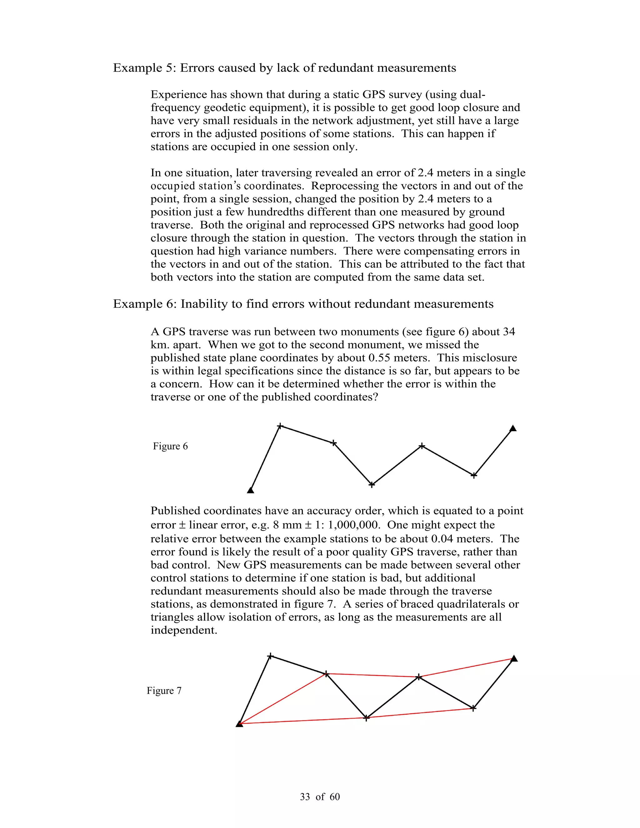
2. Analyze loop misclosures
Loop misclosures can be used to detect "bad" observations. If two loops with a
common base line have large misclosures, this may be an indication that the
common base line is an outlier. Since users must repeat base lines on different
days and at different times of the day, there are several different loops that can be
generated from the individual base lines. If a repeat base line difference is greater
than 2 cm then comparing the loop misclosures involved with the base line may
help determine which base line is the outlier. According to NGS guidelines, if a
repeat base line difference exceeds 2 cm then one of the base lines must be
observed again, and base lines must be observed at least twice on two different
days and at two different times of the day.
3. Plot ellipsoid height residuals from least squares adjustment
Like comparing repeat base lines, analyzing ellipsoid height residuals is also
important. During this procedure, the user performs a 3D minimum-constraint
least squares adjustment of the GPS survey project, i.e., constrain one latitude,
one longitude, and one ellipsoid height; plots the ellipsoid height residuals; and
investigates all residuals greater than 2 cm. Be aware that NAD 83(1998) heights
should be used since NAD 83(1991) heights are not good.
4. Select a best fit to a tilted plane
Best fitting a tilted plane to the height differences is a good method of detecting
and removing any systematic trend between the height differences. Most GPS
adjustment software available today has an option for solving for a tilted plane or
rotations and scale parameters to remove the systematic trend from data if one
exists. After a trend has been removed, all differences should be less than ± 2 cm.](https://image.slidesharecdn.com/standardsandguidelinesforlandsurveyingusinggpsver2-151019075101-lva1-app6891/75/Standards-and-guidelines-for-land-surveying-using-gps-ver-2-1-3-20-2048.jpg)
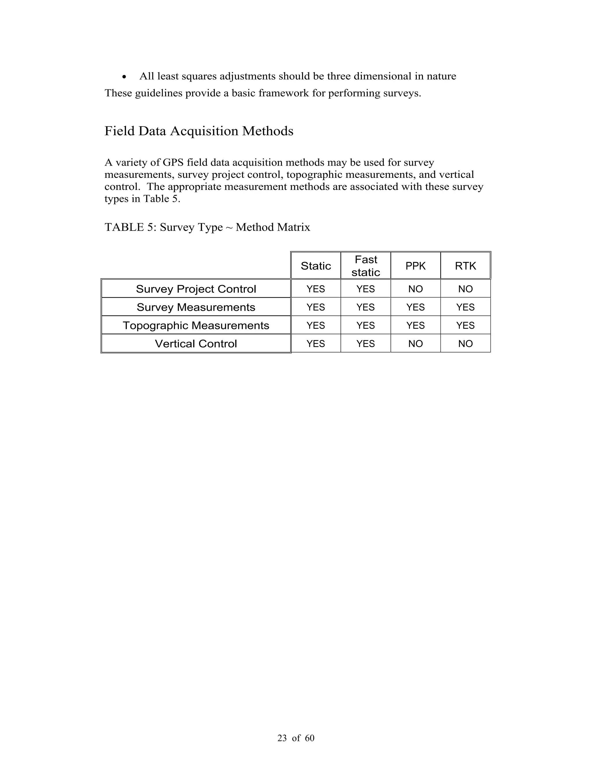


This document provides standards and guidelines for land surveying using Global Positioning System (GPS) methods in Washington State. It establishes standards for positional accuracy based on 95% confidence intervals. It describes the types of GPS surveying, field operations and procedures, data processing, and documentation requirements. The guidelines are intended to ensure surveys are repeatable, legally defensible and referenced to the National Spatial Reference System. They address eliminating error sources, observational and occupational redundancy to demonstrate accuracy, and compliance with state and federal regulations.


