gps_details.ppt

Introduction to GPS
 “… it isn’t hard to operate a GPS receiver –
matter of fact, most of them are so user-
friendly you don’t need to know the first thing
about GPS to make them work; that is, until
they don’t. Getting coordinates from a GPS
receiver is usually a matter of pushing
buttons, but knowing what those coordinates
are, and more importantly, what they aren’t,
is more difficult.”
Jan Van Sickle

Use of Satellites in Surveying
 Started as early as Sputnik (1957)
 Continued with other satellites
– Measuring positions of satellites against
background stars on photographs
– Laser ranging
– Used Doppler effect to determine velocity
vector

TRANSIT Satellite
 Navy Navigation Satellite System (NNSS) started in
1960s
 Used the Doppler shift of the signal to determine
velocity vector
 Six satellites in low (1100 km) circular, polar orbits
 One satellite every 90 minutes, need 2 passes
– Susceptible to atmospheric drag and gravitational
perturbations
– Poor quality orbital parameters
 Produces poor positions (by modern standards)

Brief History of GPS
 Initial work in 1970s
– Counselman, Shapiro, etc. (MIT)
 First used for practical purposes in 1980s
– Civilian use ahead of military use
 Initial operational capability (IOC) July ‘93
 Full operational capability (FOC) 17 July 1995

GPS Overview
 Consists of ~24 satellites
 4 satellites in 6 orbital planes
– Planes inclined 55°
 20,000 km orbits
– Periods of 11h 58m
 Each satellite carries multiple atomic clocks

GPS Segments
 User Segment
– Military and civilian users
 Space Segment
– 24 satellite constellation
 Control Segment
– Worldwide network of stations

Space Segment
 Block I
 Block II
 Block IIA (A – advanced)
 Block IIR (R – replenishment)
 Block IIF (F – Follow on)
 Block III
– See http://www.spaceandtech.com/spacedata/constellations/navstar-
gps-block1_conspecs.shtml

Control Segment
 Worldwide network of stations
– Master Control Station – Colorado Springs, CO
– Monitoring Stations – Ascension Island, Colorado
Springs, Diego Garcia, Hawaii, Kwajalein
 Other stations run by National Imagery and Mapping
Agency (NIMA)
– Ground Control Stations – Ascension, Diego
Garcia, Kwajalein

Data Flow
Master Control Station
USNO
Monitor Station
USNO
AMC
Satellite Signal
Timing
Links
Time
Timing data
Control
Data
Satellite
Signal

Basic Idea
 Broadcast signal has time embedded in it
 Need to determine distance from satellite to
receiver
 One way uses distance = velocity * time
– If time between when the signal is sent and when
it is received is known, then distance from satellite
is known
 Using multiple distances, location can be
determined (similar to trilateration)

GPS Signal Frequency
 Fundamental Frequency 10.23MHz (f0)
 2 Carrier Frequencies
– L1 (1575.42 MHz) (154 f0)
– L2 (1227.60 MHz) (120 f0)
 3 Codes
– Coarse Acquisition (C/A) 1.023 MHz
– Precise (P) 10.23 MHz
– Encrypted (Y)
 Spread Spectrum
– Harder to jam

Codes
 Stream of binary digits known as bits or
chips
– Sometimes called pseudorandom noise
(PRN) codes
 Code state +1 and –1
 C/A code on L1
 P code on L1 and L2
 Phase modulated

C/A Code
 1023 binary digits
 Repeats every millisecond
 Each satellite assigned a unique C/A-code
– Enables identification of satellite
 Available to all users
 Sometimes referred to as Standard Positioning
Service (SPS)
 Used to be degraded by Selective Availability
(SA)

P Code
 10 times faster than C/A code
 Split into 38 segments
– 32 are assigned to GPS satellites
– Satellites often identified by which part of the
message they are broadcasting
 PRN number
 Sometimes referred to as Precise Positioning
Service (PPS)
 When encrypted, called Y code
– Known as antispoofing (AS)

Future Signal
 C/A code on L2
 2 additional military codes on L1 and L2
 3rd civil signal on L5 (1176.45 MHz)
– Better accuracy under noisy and multipath
conditions
– Should improve real-time kinematic (RTK)
surveys

Time Systems
 Each satellite has multiple atomic clocks
– Used for time and frequency on satellite
 GPS uses GPS Time
– Atomic time started 6 January 1980
– Not adjusted for leap seconds
– Used for time tagging GPS signals
 Coordinated Universal Time (UTC)
– Atomic time adjusted for leap seconds to be within
±0.9 s of UT1 (Earth rotation time)

Pseudorange Measurements
 Can use either C/A- or P-code
 Determine time from transmission of
signal to when the signal is received
 Distance = time*speed of light
 Since the position of the satellite is
assumed to be known, a new position
on the ground can be determined from
multiple measurements

Carrier-phase Measurements
 The range is the sum of the number of full
cycles (measured in wavelengths) plus a
fractional cycle
– ρ = N*λ + n* λ
 The fraction of a cycle can be measured very
accurately
 Determining the total number of full cycles
(N) is not trivial
– Initial cycle ambiguity
– Once determined, can be tracked unless …

Cycle Slips
 Discontinuity or jump in phase
measurements
– Changes by an integer number
– Caused by signal loss
 Obstructions
 Radio interference
 Ionospheric disturbance
 Receiver dynamics
 Receiver malfunction

How to Fix Cycle Slips?
 Slips need to be detected and fixed
 Triple differences can aid in cycle slips
– Will only affect one of the series
 Should stand out
 Once detected, it can be fixed

GPS Errors and Biases
 Satellite Errors
– Potentially different for each satellite
 Transmission Errors
– Depends on path of signal
 Receiver Errors
– Potentially different for each receiver

Linear Combination
 Errors and biases, which cannot be
modeled, degrade the data
 Receivers that are ‘close enough’ have
very similar errors and biases
 Data can be combined in ways to
mitigate the effects of errors and biases

Linear Combination
 Combine data from two receivers to one
satellite
– Should have same satellite and
atmospheric errors
– Differences should cancel these effects out

Linear Combination
 Combine data from one receiver to two
satellites
– Should have same receiver and
atmospheric errors
– Differences should cancel these effects out

Linear Combination
 Combine data from two receivers to two
satellites
– Should have same receiver, satellite and
atmospheric errors
– Differences should cancel out

Linear Combination
 Can also combine the L1 and L2 data to
eliminate the effects of the ionosphere
– Ionosphere-free combination
 L1 and L2 phases can also be combined
to form the wide-lane observable
– Long wavelength
– Useful in resolving integer ambiguity

Two Reference Frames
 Satellites operate in an inertial
reference frame
– Best way to handle the laws of physics
 Receivers operate in a terrestrial
reference frame
– Sometimes called an Earth-centered,
Earth-fixed (ECEF) frame
– Best way to determine positions

Inertial Frame (Historically)
 X axis through the vernal equinox
 Y axis is 90° to the ‘east’
 Z axis through the Earth’s angular
momentum axis
 X-Y plane is the celestial equator
 Z axis is through the celestial North Pole

Inertial Frame
From http://celestrak.com/columns/v02n01/

Inertial Frame
 Defined by the positions of distant radio
sources called quasars
 Realization from observations provided by
Very Long Baseline Interferometry (VLBI)
– e.g. International Celestial Reference Frame
 Right-handed, Cartesian coordinate system

Terrestrial Frame (Historically)
 X axis through the Greenwich meridian
 Y axis is 90° to the east
 Z axis through the Earth’s angular
momentum axis
 X-Y plane is the equator
 Z axis is through the North Pole

Terrestrial Frame
From http://www.nottingham.ac.uk/iessg/coord1.htm

Terrestrial Frame
 Defined by the positions of reference points
 Realization from observations provided by
VLBI, SLR, and GPS
– e.g. International Terrestrial Reference Frame
– e.g. World Geodetic System (WGS)-84
 Right-handed, Cartesian coordinate system

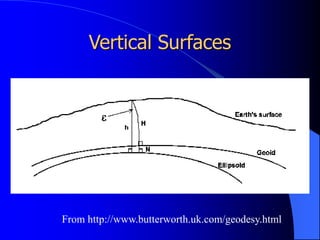
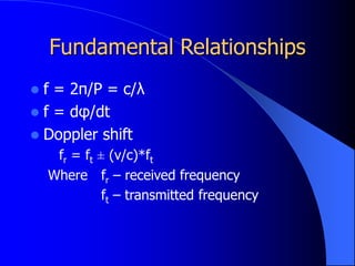
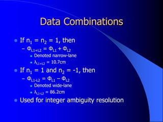
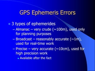
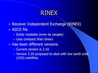
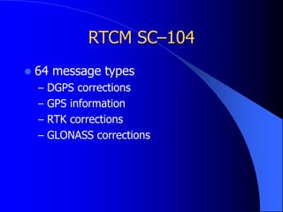
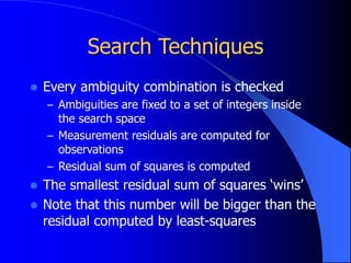
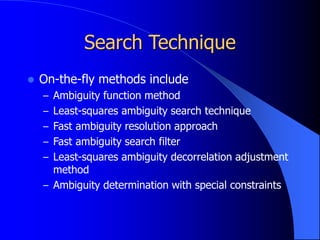
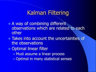
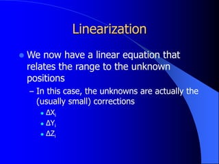
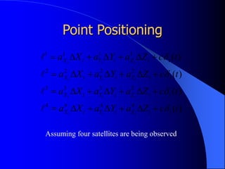
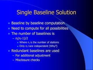
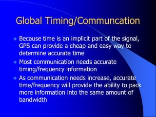
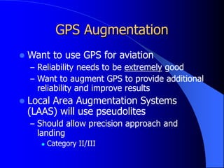
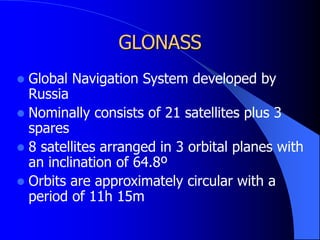
Terrestrial Frame
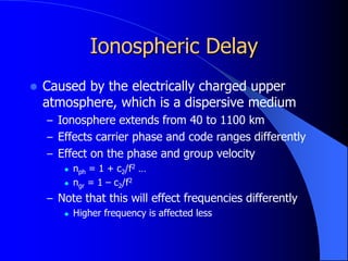
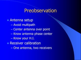
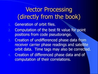
 Can transform from non-Cartesian (geodetic)
coordinates to Cartesian coordinates
– X = (N+h) cosφ cosλ
– Y = (N+h) cosφ sinλ
– Z = [ N(1-e2)+h] sin φ
 Where N = a/sqrt(1-e2sin2 φ)
 h = ellipsoid height
 φ = latitude
 λ = longitude

Transformation between
Frames
 Transformation is accomplished through
rotation by Earth orientation parameters
(EOPs)
– Polar Motion (W)
– Earth rotation (T)
– Precession/nutation (P)(N)
 xcts = (W)(T)(N)(P)xcis

Datums
 Based on a reference ellipsoid
– Semimajor axis (a) and semiminor axis (b)
or semimajor axis (a) and flattening (f)
 Needs to have a well defined center
(origin)
 Needs to have a well defined direction
or axes (orientation)

Datums
 Can be done with 8 parameters
– 2 define the ellipsoid
– 3 define the origin of the ellipsoid
– 3 define the orientation of the ellipsoid

Datums
 North American Datum 1927 (NAD27)
– Clarke ellipsoid of 1866
 North American Vertical Datum 1929
(NAVD29)
 North American Datum 1983 (NAD83)
– GRS 1980 ellipsoid
 North American Vertical Datum 1988
(NAVD88)
 Even the last two have minimal input from
GPS

Vertical Measurements
 Vertical measurements from GPS are
relative to the ellipsoid (ellipsoid height)
– Not from the geoid or topography
 To translate to other surfaces (either
reference or real) requires additional
information
– Orthometric or geoid heights

Vertical Surfaces
From http://www.butterworth.uk.com/geodesy.html

HARN
 High Accuracy Reference Network
(HARN)
 Created by states, with federal assistance
(NGS)
 Predominantly based on GPS
observations
– Very accurate

Plane Coordinate Systems
 Used over ‘local’ areas
 State Plane Coordinate (SPC) systems
– Results of projection onto surface
 Lambert conic projection
 Mercator (cylindrical) projection

Time Systems
 Earth rotation time
– Solar/sidereal
 Dynamical
– Barycenter/terrestrial
 Atomic (off by integer seconds)
– Coordinated Universal Time (UTC)
– International Atomic Time (TAI)
– GPS Time

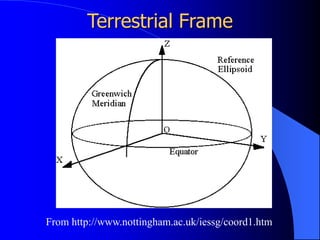
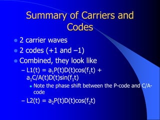
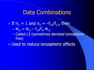
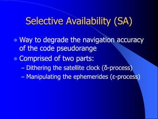
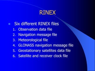
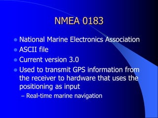
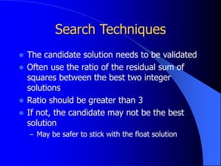
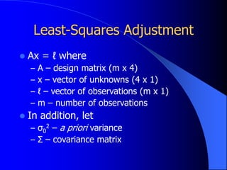
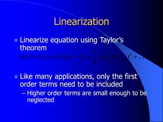
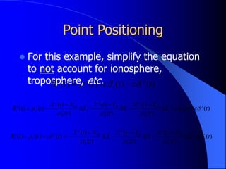
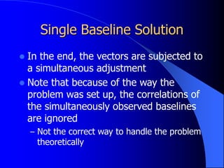
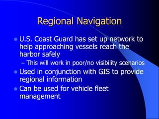
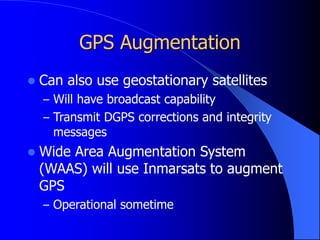
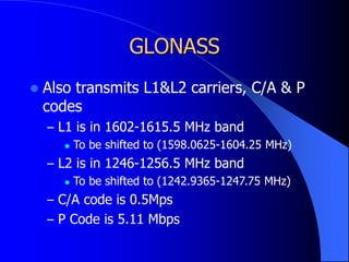
Calendar
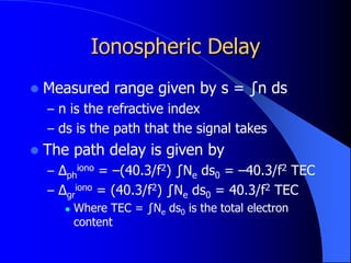
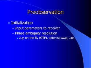
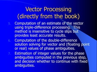
 Julian Date (JD) are days from noon (UT)
January 4713 BC
– JD = INT[365.25y] + INT[30.6001(m+1)] + D +
UT/24 + 1720981.5
 y = Y-1 and m = M+12 if M ≤ 2
 y = Y and m = M if M > 2
 Modified Julian Date
– MJD = JD – 2400000.5
– http://tycho.usno.navy.mil/mjd.html
Calculator -
http://aa.usno.navy.mil/data/docs/JulianDate.html

Kepler Orbital Parameters
(Kepler Elements)
 Ω – right ascension of ascending node
 i – inclination of orbital plane
 ω – argument of perigee
 a – semimajor axis of orbital ellipse
 e – numerical eccentricity of ellipse
 T0 – epoch of perigee passage

Kepler Elements
From
http://www.stk.com/resources/help/Data/
DemoScenarios/Training/kepler/satorbits
.htm

Perturbation of Orbits
 Mathematically, treat the problem as
small corrections to the idealized motion
 Can use mathematical tricks to simplify
the problem
– Assume the corrections are sufficiently
‘small’
– Use Taylor’s Theorem

Disturbing Accelerations
 Gravitational
– Nonsphericity of the Earth
– Tidal attraction (direct and indirect)
 Nongravitational
– Solar radiation pressure
– Relativistic effects
– Solar wind
– Magnetic field
– Out-gassing

Nonsphericity of the Earth
 The Earth’s potential can be
approximated using spherical harmonics
 Disturbing Potential can be given as
R = V – V0

Tidal Effect (direct)
 Celestial body will attract the satellite
 The effect will be a function of the angle
between the celestial body, the Earth, and the
satellite
 Only a few bodies need to be considered
– Sun
– Moon
– Venus
 Acceleration is ~10-6 m/s2

Tidal Effect (indirect)
 Celestial body will deform the Earth
– Both ocean tides and solid earth tides
 Deformation of the Earth will perturb
the orbit of the satellite

Solar Radiation Pressure
 Sunlight impinging on a surface imparts
momentum
 Two components
– Principal component away from the Sun
 Modeled
– Component along satellite y-axis (y-bias)
 Solved for
 Eclipse ‘season’ causes additional problems

Relativistic Effect
 Caused by the Earth’s gravity field
 Creates a perturbing acceleration

Other
 Solar Wind
– Sun emits a wind which interacts with
objects in the solar system
 Magnetic Field
– Interaction of the Earth’s magnetic field
with a (metallic) satellite
 Out-gassing
– Gasses from satellite evaporate
– Act similar to a jet

Orbit Dissemination
 Best orbital determinations come from a
global network with a ‘good’ geometric
distribution
– Want ~30 stations if possible
 Military network
– Monitoring Stations
 Civilian
– International GPS Service (IGS)

Types of Orbits
 Almanac
– Poor quality (~100m)
– Used well into the future
 Broadcast
– Good quality (1-2m with SA off)
– Used in real-time work
 Precise
– Excellent quality (5-10cm)
– Used in the most precise work

Fundamental Relationships
 f = 2π/P = c/λ
 f = dφ/dt
 Doppler shift
fr = ft ± (v/c)*ft
Where fr – received frequency
ft – transmitted frequency

Summary of Carriers and
Codes
 2 carrier waves
 2 codes (+1 and –1)
 Combined, they look like
– L1(t) = a1P(t)D(t)cos(f1t) +
a1C/A(t)D(t)sin(f1t)
 Note the phase shift between the P-code and C/A-
code
– L2(t) = a2P(t)D(t)cos(f2t)

C/A Code
 Produced by 2 10-bit feedback shift
registers
 Frequency is 1.023 MHz
 Repetition rate of 1ms
 The code length is 1023 chips
 Time interval between 2 chips is 1μs
– 300 m chip length

P Code
 Produced by 2 shift registers
 The code length is 2.3547*1014 bits
 Corresponding time span is 266.4 days
 Chip length is 30 m
 To protect against deliberate misinformation,
combined with the encrypting W-code to
produce Y-code
– Only accessible if you know how to decode (i.e.
military applications)

Navigation Message
 Contains information about each satellite
– Clocks, orbits, health, corrections
 Subframes contain
– Telemetry word (TLM)
– Hand-over word (HOW)
– Clock Corrections
– Broadcast ephemeris
– Almanac data

Signal Processing
 Different inputs (codes, NAV message,
carriers) get combined
 Combined signal is broadcast by satellite
 Receiver picks up broadcast and must
decompose the signal to recover
– Code
– Navigation message
– Carrier

Receivers
 Must contain
– Signal reception (antenna)
 Omnidirectional
 Signals measured from phase center
– Signal processing
 Microprocessor controls system
 Control device provides communications
 Storage device

Radio Frequency Signal
 Need to discriminate between satellites
– Use unique codes
– Use unique Doppler shifts
 Modern receivers use a separate channel for
each satellite (continuous tracking)
 Receivers also need to be able to generate
frequency to create their own signals
– Usually uses internal oscillator

How to Determine Time?
 PRN code generated on satellite
 Identical code created in receiver
 If the time on the satellite were
synchronized to the receiver, problem
solved
– Unfortunately, not the case
 Trick is to match up the code to find time
 Use autocorrelation




1
0
)
(
)
(
1
)
(
N
t
x
t
x
N
r 


Additional Techniques
 Squaring technique
 Cross correlation technique
 Code correlation plus squaring
technique
 Z-tracking technique

Code Squaring
 Used to eliminate code information
– Results consist only of carrier wave
 Multiply the modulated carrier by itself
(square the signal)
 Code signal (which consists of +1 and –
1) becomes 1 throughout
– (+1)2 = 1
– (-1)2 = 1

Data
 Code Pseudorange
 Carrier Phase
 Doppler
 Combinations of data
 Biases and Noise terms

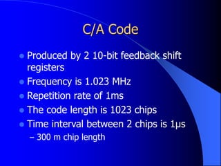
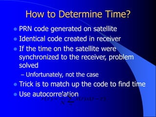
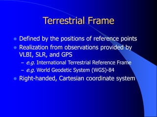
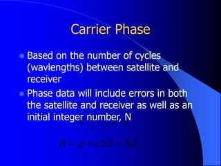
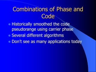
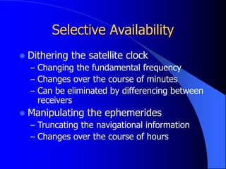
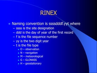
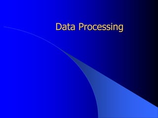
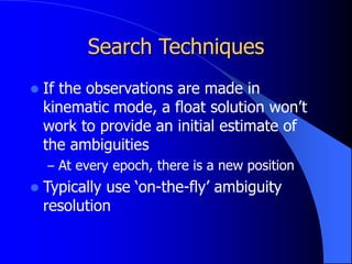
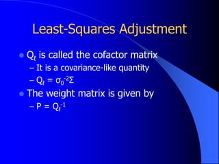
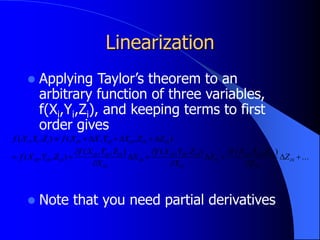
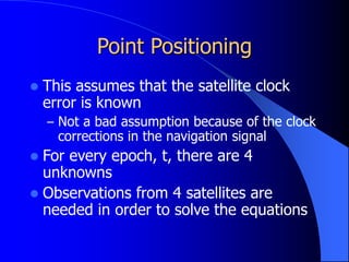
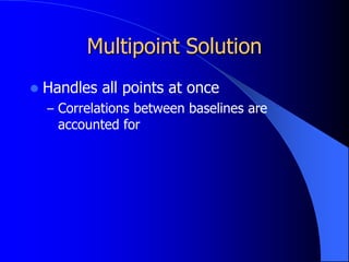
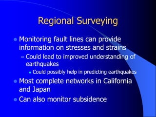
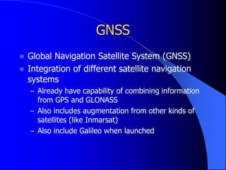
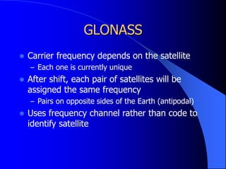
Code Pseudorange
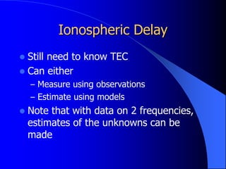
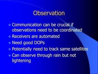
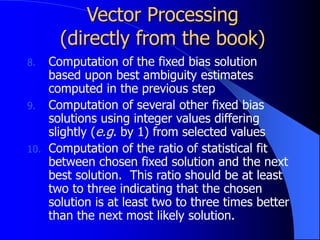
 Based on travel time between when
signal is sent and when it is received
 Time data also includes errors in both
satellite and receiver clocks
– Δt = tr – ts = [tr(GPS)-δr] – [ts(GPS) – δs]
 Pseudorange given by R = c Δt = ρ +
cΔδ
– Pseudo because of cΔδ (where Δδ = δs – δr)
factor

Carrier Phase
 Based on the number of cycles
(wavlengths) between satellite and
receiver
 Phase data will include errors in both
the satellite and receiver as well as an
initial integer number, N
N
c




 





 N
c
R 




Doppler
 Doppler shift depends on radial velocity
– More useful for determining velocities than
for determining positions
 To get positions, need to integrate
Doppler shifts (phase differences)


 



 c
dt
d
dt
d
D

Data Combinations
 Theoretically, data can be obtained
from
– Code ranges – RL1, RL2
– Carrier phases – ΦL1, ΦL2
– Doppler shifts – DL1, DL2
 Combinations of these data could be
used as well

Data Combinations
 In general, linear combinations of phase
will look like
– φ = n1φ1 + n2φ2
– Where n1 and n2 can be any integer
 Noise level increases for combined data
– Assuming noise levels are equal for both,
the increase is by a factor of √2

Data Combinations
 If n1 = n2 = 1, then
– ΦL1+L2 = ΦL1 + ΦL2
 Denoted narrow-lane
 λL1+L2 = 10.7cm
 If n1 = 1 and n2 = -1, then
– ΦL1-L2 = ΦL1 – ΦL2
 Denoted wide-lane
 λL1-L2 = 86.2cm
 Used for integer ambiguity resolution

Data Combinations
 If n1 = 1 and n2 = –fL2/fL1, then
– ΦL3 = ΦL1 – fL2/fL1 ΦL2
– Called L3 (sometimes denoted ionosphere-
free)
 Used to reduce ionospheric effects

Combinations of Phase and
Code
 Historically smoothed the code
pseudorange using carrier phase
 Several different algorithms
 Don’t see as many applications today

What to do with Errors?
 There are essentially 4 options:
– Ignore them
 Works if the errors are small (negligible)
– Model them
 Need good models
 Not all effects can be modeled
– Solve for them
 Increases complexity of solution
– Make them go away

GPS Ephemeris Errors
 3 types of ephemerides
– Almanac – very crude (~100m), used only
for planning purposes
– Broadcast – reasonably accurate (~1m),
used for real-time work
– Precise – very accurate (~10cm), used for
high precision work
 Available after the fact

Selective Availability (SA)
 Way to degrade the navigation accuracy
of the code pseudorange
 Comprised of two parts:
– Dithering the satellite clock (δ-process)
– Manipulating the ephemerides (ε-process)

Selective Availability
 Dithering the satellite clock
– Changing the fundamental frequency
– Changes over the course of minutes
– Can be eliminated by differencing between
receivers
 Manipulating the ephemerides
– Truncating the navigational information
– Changes over the course of hours

Clock Errors
 Both satellites and receivers will have clock
errors
– There’s no such thing as a perfect clock
 Any error in a clock will propagate directly into
a positioning error
– Remember distance = velocity*time
 Satellite clock errors can be reduced by
applying the corrections contained in the
broadcast

Ionospheric Delay
 Caused by the electrically charged upper
atmosphere, which is a dispersive medium
– Ionosphere extends from 40 to 1100 km
– Effects carrier phase and code ranges differently
– Effect on the phase and group velocity
 nph = 1 + c2/f2 …
 ngr = 1 – c2/f2
– Note that this will effect frequencies differently
 Higher frequency is affected less

Ionospheric Delay
 Measured range given by s = ∫n ds
– n is the refractive index
– ds is the path that the signal takes
 The path delay is given by
– Δph
iono = –(40.3/f2) ∫Ne ds0 = –40.3/f2 TEC
– Δgr
iono = (40.3/f2) ∫Ne ds0 = 40.3/f2 TEC
 Where TEC = ∫Ne ds0 is the total electron
content

Ionospheric Delay
 Still need to know TEC
 Can either
– Measure using observations
– Estimate using models
 Note that with data on 2 frequencies,
estimates of the unknowns can be
made

Tropospheric Delay
 Caused by the neutral atmosphere, which is a
nondispersive medium (as far as GPS is
concerned)
– Troposphere extends up to 40 km
– Effects carrier phase and code ranges the same
 Typically separate the effect into
– Dry component
– Wet component
 ΔTrop = 10-6∫Nd
Trop ds + 10-6∫Nw
Trop ds
– Where N is the refractivity
– ds is the path length

Tropospheric Delay
 Dry component contributes 90% of the
error
– Easily modeled
 Wet component contributes 10% of the
error
– Difficult to model because you need to
know the amount of water vapor along the
entire path

Tropospheric Delay
 There are many models which estimate the
wet component of the tropospheric delay
– Hopfield Model
– Modified Hopfield Model
– Saastamoinen Model
– Lanyi Model
– NMF (Niell)
– Many, many more

Special Relativistic
Considerations
 Time dilation
– Moving clock runs slow
 Lorentz contraction
– Moving object seems contracted
 Second order Doppler effect
– Frequency is modified like time
 Mass relation

General Relativistic
Considerations
 Perturbations in the satellite orbit
 Curvature of the path of the signal
– Longer than expected in Euclidian space
 Effects on the satellite clock
– Clocks run fast further out of the potential
well
 Effects on the receiver clock (Sagnac
effect)

Phase Center Errors
 Phase center is the ‘point’ from which the
GPS location is measured
 Difficult to measure precisely
 Changes with different factors:
– Elevation
– Azimuth
– Frequency
 Either model the error or reduce the effect of
the error by always orienting antenna the
same direction

Receiver Noise
 All electronic devices will have a certain
amount of noise
 Because of the characteristics of the
noise modeling is not an option
 The best that can be done is average
the data to reduce the effects of the
noise

Multipath Errors
 GPS assumes that the signal travels
directly from the satellite to the receiver
 Multipath results from signal reflecting
off of surface before entering the
receiver
– Adds additional (erroneous) path length to
the signal
 Difficult to remove; best to avoid

Multipath Illustration
From
http://www.gmat.unsw.edu.au/snap/gps/gps_survey/chap6/6212.htm

Geometric Factors
 The strength of figure of the satellites is
taken into consideration by the dilution
of precision (DOP) factor
– Depends on number of satellites
– Depends on location of satellites

Geometric Factors
From http://www.romdas.com/surveys/sur-gps.htm

Geometric Factors
 Different kinds of DOPs
– HDOP (horizontal)
– VDOP (vertical)
– PDOP (position) (3-D component)
– TDOP (time)
– GDOP (geometric) (PDOP and TDOP)

User Equivalent Range Error
(UERE)
 Crude estimate of the expected error
 Consists of contributions from
– Measurement noise
– Satellite biases
– Wave propagation errors
 Transmitted through the Navigation
message
 Combined with DOP information

General Thoughts on Survey
 Accuracy
 Project size
 Density of control
 Physical restrictions
 Number of receivers
 Adjustment capability
 Station and reference azimuth mark visibility
 Cost
 Observation time

More Specific Thoughts
 Code range vs. carrier phase
 Real-time processing vs. postprocessing
 Point positioning vs. relative positioning
 Static vs. kinematic

Observation Techniques
 Point Positioning
 Differential GPS
 Relative Positioning

Point Positioning
 Determines the coordinates of the receiver
 If using a single receiver, this is the only reasonable
option
 Standard Positioning Service (SPS) uses C/A code
– ~10 m accuracy
 Precise Positioning Service (PPS) uses both codes
– ~1 m accuracy

Differential GPS
 Uses (at least) two receivers
– One located at a known point
– One used to determine position of unknown point
 Typically uses pseudorange data
 Known position used to compute corrections
 At least four common satellites must be observed

Differential GPS
 Correction transmitted to other receiver
– Need to have a (radio) data link
 Data usually transmitted using the Radio
Technical Commission for Maritime Service,
Special Committee 104 (RTCM) format
 Initial position combined with correction to
create a refined position

Relative Positioning
 Uses (at least) two receivers
– One located at a known point
– One used to determine position of
unknown point
 Typically uses carrier phase
 Determine the vector between known
point and unknown point

 Static
– Receivers remain stationary
 Rapid Static
– Receivers remain stationary for short times
– Need good receivers (dual frequency)

 Kinematic
– Receiver is continually moving
– Must maintain lock on 4 satellites at all times
 Semi-kinematic (stop-and-go)
– Receiver makes brief stops
 Pseudokinematic
– Receiver makes stops but must reoccupy after
significant (~1 hour) time

Field Equipment
 Typical equipment includes (but not limited
to)
– Receiver
– Battery
– Meteorological sensor
– Tripod
– Tribrach
– Communication device

Survey Planning
 Decide the extent of the planning
 Study a map of the area
 Point selection
 Satellite coverage
– DOP estimates
 Session length
 Field reconnaissance

Survey Planning
 Monumentation
 Organizational Design
– Personnel
– Vehicles
– Equipment
– Sites

Organizational Design
 Number of sessions
– n = (s-o)/(r-o)
 s – number of sites
 r – number of receivers
 o – overlapping sites
– n = ms/r
 m – number of times site to be occupied

Organizational Design
 Radial survey
– One receiver placed at fixed site
– Other receivers placed at locations
– Measure lines from fixed site to other
locations
 Network survey
– Closed geometric figures

Surveying Procedure
 Preobservation
 Observation
 Postobservation
 Ties to control monument

Preobservation
 Antenna setup
– Avoid multipath
– Center antenna over point
– Know antenna phase center
– Know your H.I.
 Receiver calibration
– One antenna, two receivers

Preobservation
 Initialization
– Input parameters to receiver
– Phase ambiguity resolution
 e.g. on-the-fly (OTF), antenna swap, etc.

Observation
 Communication can be crucial if
observations need to be coordinated
 Receivers are automated
 Need good DOPs
 Potentially need to track same satellites
 Can observe through rain but not
lightening

Survey Procedure
 Postobservations
– Document!
 Prepare site occupation sheet
 Ties to the control monuments
– Usually need to connect the survey to
control

Data Processing
 Transfer the data to computer
 Process the data
– Use ‘canned’ software
– Two strategies for static surveys
 Vector-by-vector (single baseline)
– Easier to detect bad baselines
 Mulitpoint solutions
– Not as common

Vector Processing
(directly from the book)
1. Generation of orbit files.
2. Computation of the best fit value for point
positions from code pseudorange.
3. Creation of undifferenced phase data from
receiver carrier phase readings and satellite
orbit data. Time tags may also be corrected.
4. Creation of differenced phase data and of
computation of their correlations.

Vector Processing
5. Computation of an estimate of the vector
using triple-difference processing. This
method is insensitive to cycle slips but
provides least accurate results.
6. Computation of the double-difference
solution solving for vector and (floating point
or real) values of phase ambiguities.
7. Estimation of integer values for the phase
ambiguities computed in the previous step,
and decision whether to continue with fixed
ambiguities.

Vector Processing
8. Computation of the fixed bias solution
based upon best ambiguity estimates
computed in the previous step
9. Computation of several other fixed bias
solutions using integer values differing
slightly (e.g. by 1) from selected values
10. Computation of the ratio of statistical fit
between chosen fixed solution and the next
best solution. This ratio should be at least
two to three indicating that the chosen
solution is at least two to three times better
than the next most likely solution.

Troubleshooting
 Easiest to see with single baseline
vectors
 Check standard error estimates
 Check ratio
 Check rms
 Check ambiguities

Network Adjustment
 Check loop closures
 Perform minimally constrained least-squares
solution
– Bad lines must be removed first
– Check computed coordinates with previous
 Points with large shifts could be problematic
 Check residuals (both normalized and
unnormalized)
 Scale errors by appropriate factor

And Finally …
 Transform coordinates into appropriate
coordinate system
 Produce final report
– Formats will differ depending on employer
– See book for an example of things to
consider

Formats
 Each receiver stores data in its own
(proprietary) binary format
– Saves space
 Combining data from different receivers
could potentially be problematic
 Need standard formats that are
supported by different equipment

Formats
 RINEX
 NGS-SP3
 RTCM SC-104
 NMEA 0183

RINEX
 Receiver Independent Exchange (RINEX)
 ASCII file
– Easily readable (even by people)
– Less compact than binary
 Has been different versions
– Current version is 2.10
– Version 2.20 proposed to deal with low earth orbit
(LEO) satellites

RINEX
 Six different RINEX files
1. Observation data file
2. Navigation message file
3. Meteorological file
4. GLONASS navigation message file
5. Geostationary satellites data file
6. Satellite and receiver clock file

RINEX
 Naming convention is ssssdddf.yyt where
– ssss is the site designation
– ddd is the day of year of the first record
– f is the file sequence number
– yy is the two digit year
– t is the file type
 O – observation
 N – navigation
 M – meteorological
 G – GLONASS
 H – geostationary

RINEX
 Observation files
– Header
 Information on observing session
– Data
 Divided into epochs

RINEX
 Navigation file
– Header
– Data
 Clock parameters
 Broadcast orbit
 Meteorological file
– Header
– Data
 Temperature
 Barometric Pressure
 Relative Humidity

NGS-SP3
 National Geodetic Survey – Standard
Product #3
 ASCII file
 Facilitates exchanging precise satellite
ephemerides

NGS-SP3
 Header
– Information on observing session (date,
number of satellites,
 Data
– Divided into epochs
– Each satellite on a separate line
 Satellite orbits, clock corrections

RTCM SC–104
 Radio Technical Commission for
Maritime Services, Special Committee
104
 Original format used for transmitting
information for real-time DGPS
– Differential corrections
 Current version 2.2

RTCM SC–104
 64 message types
– DGPS corrections
– GPS information
– RTK corrections
– GLONASS corrections

NMEA 0183
 National Marine Electronics Association
 ASCII file
 Current version 3.0
 Used to transmit GPS information from
the receiver to hardware that uses the
positioning as input
– Real-time marine navigation

Data Handling
 Downloading
– Need to move data from receiver to computer
 Data Management
– Need structure to handle large amounts of data
– Separating by projects is often used
 Data Exchange
– Original data usually binary
– May want data in other formats
 Most receivers now convert to Receiver Independent
Exchange (RINEX) format

Cycle Slips
 When a receiver is turned on, there is an
initial integer number of wavelengths (Nj) for
every satellite j when measuring carrier phase
 When a receiver loses lock on a particular
satellite, there is a new initial integer number
of wavelengths (Nj*) for every satellite j
– This event is called a cycle slip
– Note that Nj ≠ Nj*
 Unfortunately, the receiver/software assumes
that Nj is a constant unless told otherwise
– Produces a sudden apparent jump in position

Cycle Slips
 Generally caused by one of four things
– Obstructions
 Caused by trees, buildings, bridges, mountains, etc.
 Most frequent problem
– Low signal-to-noise (SNR) ratio
 Caused by ionospheric conditions, multipath, high
receiver dynamics, low satellite elevations
– Failure in receiver software
 Infrequent
– Malfunctioning satellite oscillators
 Rare

Cycle Slips
http://www.gmat.unsw.edu.au/snap/gps/gps_survey/chap7/735.htm

Cycle Slips
 Need to determine the instant at which
the slip occurs
– Accomplished by comparing observations
at successive epochs
– Often done using triple differences
 ‘Repairs’ consist of correcting all
subsequent observations for the jump
– Note that the jump must be an integer

Ambiguity Resolution
 Assuming that tracking is continuous,
there is no time dependence to
equations
– Φ = λ-1ρ + fΔδ + N – λ-1ΔIono
– Need to determine integer ambiguity N
 Once accomplished, ambiguity is said to be
resolved or fixed
 Note that ambiguity resolution is not
always a possibility

 For instance, look at double differences
– λΦ = ρAB
jk(t) + λN + noise
– Effect of ionosphere, troposphere are
neglected
 Any errors from these terms will
contaminate the parameter estimation
– The ‘best’ estimates (think least-squares) for
N may not be an integer even though they
should be

 Satellite geometry is an important
consideration
– More satellites with better geometry will
provide better DOPs
– Better DOPs will improve ambiguity resolution
 Length of observation critical to ambiguity
resolution
– Want to track the satellite across the sky

 Multipath can make ambiguity
resolution more difficult
– It contaminates observations which makes
parameter estimation more difficult

 Three steps need to followed
– Determine the ‘search space’
– Identify the correct integers
– Validation of integer set

 Determine the ‘search space’
– Which integers could possibly be correct?
 Remember that the problem is multi-dimensional
 Every satellite will have an integer ambiguity
– Since the solution will be pulled from the search
space, you need to be conservative to ensure that
the correct integers will be selected
– However, the bigger the search space, the longer
it will take to find the integers
– In static positioning, can be determined
approximately from float solution

 Identify the correct integers
– Done statistically
– Minimizing sum of squared residuals
– Assume that the integers that best fit the
observations are most likely to be correct
– Also assumes that the integers are normally
distributed
 Not always true
 Most frequent cause of resolution failure in long
baselines

 Validation of integer set
– How correct are the integers selected?
– Success rate depends on
 Observation equations
 Precision of observables
 Method of estimation
– Are the integers chosen significantly better
than the other possibilities
 Look at ratio of the sum of squared residuals
 Want the ratio to be three or greater

Approaches
 Single frequency phase data
 Dual frequency phase data
 Combining dual frequency carrier phase
and code data
 Combining triple frequency carrier
phase and code data
– Only after modernization

Search Techniques
 If processing double-differences by
least-squares, the initial estimates of
ambiguities are real (floating point)
numbers
– Called a float solution
 Produces ‘best estimate’ of ambiguities

Search Techniques
 However, the results won’t be correct because
the numbers won’t be integers
 They will be close if
– Stations are close together
– Observation span is long
 If the two results are close, the resulting
differences in position should be close
 Otherwise, ambiguity resolution is more
important

Search Techniques
 For the static case, the search space can be
created from the float ambiguity solution and
statistics
– Take the float solution estimate and use the
standard deviations to indicate how big a window to
use
– Typically use 3σ windows
 The number of possibilities increases quickly
with the uncertainty and number of satellites

Search Techniques
 Every ambiguity combination is checked
– Ambiguities are fixed to a set of integers inside
the search space
– Measurement residuals are computed for
observations
– Residual sum of squares is computed
 The smallest residual sum of squares ‘wins’
 Note that this number will be bigger than the
residual computed by least-squares

Search Techniques
 The candidate solution needs to be validated
 Often use the ratio of the residual sum of
squares between the best two integer
solutions
 Ratio should be greater than 3
 If not, the candidate may not be the best
solution
– May be safer to stick with the float solution

Search Techniques
 If the observations are made in
kinematic mode, a float solution won’t
work to provide an initial estimate of
the ambiguities
– At every epoch, there is a new position
 Typically use ‘on-the-fly’ ambiguity
resolution

Search Technique
 Can use code solution to estimate position
– Need a good receiver
– The search space will be larger than for static case
because of the increased uncertainties
 Use wide-lane to get a better estimate of the
position
– Smaller search space
 Use improved position for final ambiguity
resolution

Search Technique
 On-the-fly methods include
– Ambiguity function method
– Least-squares ambiguity search technique
– Fast ambiguity resolution approach
– Fast ambiguity search filter
– Least-squares ambiguity decorrelation adjustment
method
– Ambiguity determination with special constraints

Least-Squares Adjustment
 Ax = ℓ where
– A – design matrix (m x 4)
– x – vector of unknowns (4 x 1)
– ℓ – vector of observations (m x 1)
– m – number of observations
 In addition, let
– σ0
2 – a priori variance
– Σ – covariance matrix

 Qℓ is called the cofactor matrix
– It is a covariance-like quantity
– Qℓ = σ0
-2Σ
 The weight matrix is given by
– P = Qℓ
-1

 To get a consistent solution, noise is added
– ℓ + n = Ax
 A unique solution can be found with
– nTPn = minimum
– ATPAx = ATPℓ
– x = (ATPA)-1ATPℓ
– Qx = (ATPA)-1 (from covariance propagation)

Kalman Filtering
 A way of combining different
observations which are related to each
other
 Takes into account the uncertainties of
the observations
 Optimal linear filter
– Must assume a linear process
– Optimal in many statistical senses

Linearization
 Linearize equation using Taylor’s
theorem
 Like many applications, only the first
order terms need to be included
– Higher order terms are small enough to be
neglected
...
)
)(
(
2
1
)
)(
(
)
(
)
( 2
0
0
0
0
0 




 t
t
t
x
t
t
t
x
t
x
t
x 



Linearization
 Applying Taylor’s theorem to an
arbitrary function of three variables,
f(Xi,Yi,Zi), and keeping terms to first
order gives
 Note that you need partial derivatives
...
)
,
,
(
)
,
,
(
)
,
,
(
)
,
,
(
)
,
,
(
)
,
,
(
0
0
0
0
0
0
0
0
0
0
0
0
0
0
0
0
0
0
0
0
0
0
0





















i
i
i
i
i
i
i
i
i
i
i
i
i
i
i
i
i
i
i
i
i
i
i
i
i
i
Z
Z
Z
Y
X
f
Y
Y
Z
Y
X
f
X
X
Z
Y
X
f
Z
Y
X
f
Z
Z
Y
Y
X
X
f
Z
Y
X
f

Linearization
2
2
2
)
)
(
(
)
)
(
(
)
)
(
(
)
( i
j
i
j
i
j
j
i Z
t
Z
Y
t
Y
X
t
X
t 






)
(
)
(
)
,
,
(
0
0
0
0
0
0
t
X
t
X
X
Z
Y
X
f
j
i
i
j
i
i
i
i






)
(
)
(
)
,
,
(
0
0
0
0
0
0
t
Y
t
Y
Y
Z
Y
X
f
j
i
i
j
i
i
i
i






)
(
)
(
)
,
,
(
0
0
0
0
0
0
t
Z
t
Z
Z
Z
Y
X
f
j
i
i
j
i
i
i
i






Z
t
Z
t
Z
Y
t
Y
t
Y
X
t
X
t
X
t
t j
i
i
j
i
j
i
i
j
i
j
i
i
j
j
i
j
i 









)
(
)
(
)
(
)
(
)
(
)
(
)
(
)
(
0
0
0
0
0
0
0






Linearization
 We now have a linear equation that
relates the range to the unknown
positions
– In this case, the unknowns are actually the
(usually small) corrections
 ΔXi
 ΔYi
 ΔZi

Point Positioning
 For this example, simplify the equation
to not account for ionosphere,
troposphere, etc. )
(
)
(
)
(
)
( t
c
t
c
t
t
R j
i
j
i
j
i 

 


)
(
)
(
)
(
)
(
)
(
)
(
)
(
)
(
)
(
)
(
0
0
0
0
0
0
t
c
t
c
Z
t
Z
t
Z
Y
t
Y
t
Y
X
t
X
t
X
t
t
R j
i
i
j
i
i
j
i
j
i
i
j
i
j
i
i
j
j
i
j
i 




 











)
(
)
(
)
(
)
(
)
(
)
(
)
(
)
(
)
(
)
(
0
0
0
0
0
0
t
c
Z
t
Z
t
Z
Y
t
Y
t
Y
X
t
X
t
X
t
c
t
t
R i
i
j
i
i
j
i
j
i
i
j
i
j
i
i
j
j
j
i
j
i 




 













Point Positioning
 This assumes that the satellite clock
error is known
– Not a bad assumption because of the clock
corrections in the navigation signal
 For every epoch, t, there are 4
unknowns
 Observations from 4 satellites are
needed in order to solve the equations

Point Positioning
)
(
)
(
)
(
)
(
)
(
)
(
)
(
)
(
)
(
0
0
0
0
0
0
0
t
Z
t
Z
a
t
Y
t
Y
a
t
X
t
X
a
t
c
t
t
R
j
i
i
j
j
X
j
i
i
j
j
Y
j
i
i
j
j
X
j
j
i
j
i
j
i
i
i



















Point Positioning
)
(
)
(
)
(
)
(
4
4
4
4
3
3
3
3
2
2
2
2
1
1
1
1
t
c
Z
a
Y
a
X
a
t
c
Z
a
Y
a
X
a
t
c
Z
a
Y
a
X
a
t
c
Z
a
Y
a
X
a
i
i
Z
i
Y
i
X
i
i
Z
i
Y
i
X
i
i
Z
i
Y
i
X
i
i
Z
i
Y
i
X
i
i
i
i
i
i
i
i
i
i
i
i




































Assuming four satellites are being observed

Point Positioning















c
a
a
a
c
a
a
a
c
a
a
a
c
a
a
a
A
i
i
i
i
i
i
i
i
i
i
i
i
Z
Y
X
Z
Y
X
Z
Y
X
Z
Y
X
4
4
4
3
3
3
2
2
2
1
1
1
















)
(t
Z
Y
X
x
i
i
i
i
 














4
3
2
1





Ax



Other Observations
 Analogously, can set up equations for
carrier phase
– (or Doppler, or combinations, etc.)
 Can also set up equations for relative
positioning

Network Adjustment
 There are two methods of determining
positions of a network
– Single baseline solution
– Multipoint solution

Single Baseline Solution
 Baseline by baseline computation
 Need to compute for all possibilities
 The number of baselines is
– ni(ni-1)/2
 Where ni is the number of stations
 Only ni-1are independent (Why?)
 Redundant baselines are used
– For additional adjustment
– Misclosure checks

Single Baseline Solution
 In the end, the vectors are subjected to
a simultaneous adjustment
 Note that because of the way the
problem was set up, the correlations of
the simultaneously observed baselines
are ignored
– Not the correct way to handle the problem
theoretically

Multipoint Solution
 Handles all points at once
– Correlations between baselines are
accounted for

Single Baseline vs. Multipoint
(from text)
 Correlations not modeled correctly with the
single baseline solution
 Computer program simpler for single baseline
 Computation time not an issue
 Cycle slips easier to detect and repair in
multipoint solution
 Easier to isolate (and eliminate) bad
measurements in single baseline
 Correlations with multipoint while better than
single baseline still might not be perfect

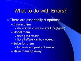
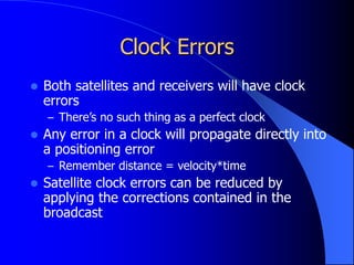
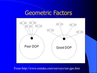
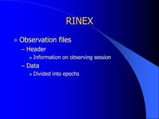
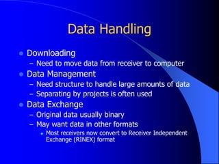
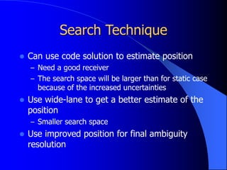
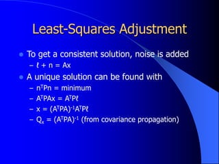
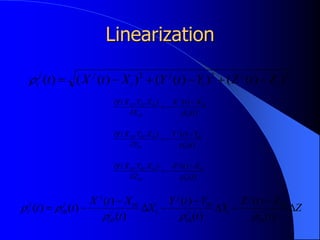
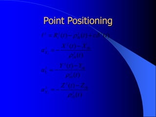
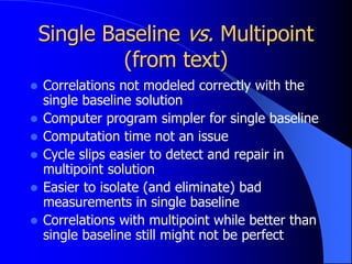
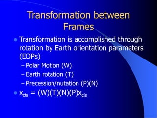
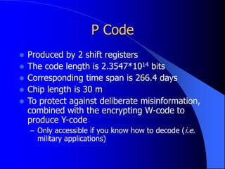
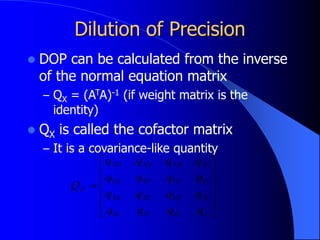
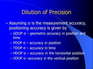
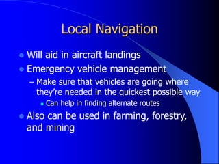
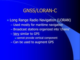
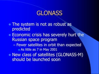
Dilution of Precision
 The dilution of precision (DOP) is a
measure of the geometry of the
satellites
 It changes with time
– Number of satellites changes
– Position of satellites changes


















































c
t
Z
Z
t
Y
Y
t
X
X
c
t
Z
Z
t
Y
Y
t
X
X
c
t
Z
Z
t
Y
Y
t
X
X
c
t
Z
Z
t
Y
Y
t
X
X
A
i
i
i
i
i
i
i
i
i
i
i
i
i
i
i
i
i
i
i
i
i
i
i
i
)
(
)
(
)
(
)
(
)
(
)
(
)
(
)
(
)
(
)
(
)
(
)
(
4
0
0
4
4
0
0
4
4
0
0
4
3
0
0
3
3
0
0
3
3
0
0
3
2
0
0
2
2
0
0
2
2
0
0
2
1
0
0
1
1
0
0
1
1
0
0
1













 The first three elements in each row are
components of the unit vector pointing
from the four satellites to the observing
site i
 Solution exists as long as the design
matrix (A) is non-singular
– The determinant is not zero

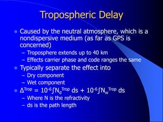
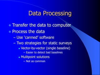
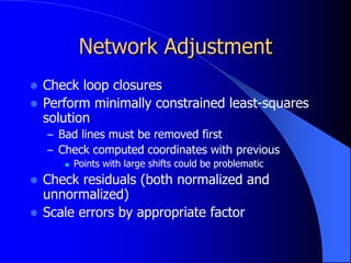
 The determinant is proportional to the
scalar triple product
 The scalar triple product is one way to
compute the volume of a body defined
by the three vectors
)
(
)]
(
)
[( 1
2
1
3
1
4
i
i
i
i
i
i 




 





 The larger the volume, the better the
geometry
 The better the geometry, the lower the
value of DOP
 Therefore, want DOP to be inversely
proportional to the volume

 DOP can be calculated from the inverse
of the normal equation matrix
– QX = (ATA)-1 (if weight matrix is the
identity)
 QX is called the cofactor matrix
– It is a covariance-like quantity













tt
tZ
tY
tX
Zt
ZZ
ZY
ZX
Yt
YZ
YY
YX
Xt
XZ
XY
XX
X
q
q
q
q
q
q
q
q
q
q
q
q
q
q
q
q
Q

tt
ZZ
YY
XX
tt
ZZ
YY
XX
q
TDOP
q
q
q
PDOP
q
q
q
q
GDOP








Note that these are expressed in the equatorial system

 Similar quantities can be calculated for
the topocentric local coordinate system
– Axes along local north, east, and up
 The global cofactor matrix QX needs to
be transformed into the local cofactor
matrix Qx
– Use the law of covariance propagation













hh
hy
hx
yh
yy
yx
xh
xy
xx
T
X
x
q
q
q
q
q
q
q
q
q
R
RQ
Q
 T
u
e
n
R 

 The three dimensional error, whether
computed in the equatorial coordinate
system or the local coordinate system
must be the same
 However
– qXX ≠ qxx
– qYY ≠ qyy hh
yy
xx
q
VDOP
q
q
HDOP




 Assuming σ is the measurement accuracy,
positioning accuracy is given by
– GDOP σ – geometric accuracy in position and
time
– PDOP σ – accuracy in position
– TDOP σ – accuracy in time
– HDOP σ – accuracy in the horizontal position
– VDOP σ –accuracy in the vertical position

Integration
 GPS determines positions
– Can provide a lot of input in a short
amount of time
 Many other systems can use positions
as inputs
– Either real-time or post-processed
 GPS and other technology make a good
match

GPS/GIS
 Geographic information system (GIS)
– Acquires, stores, manipulates, analyzes,
and displaying spatially oriented data
– Data stored in layers
 GIS is a tool to study the geographic
information
– Coordinates can be provided by GPS

GPS/GIS
 Industries that use this combination
include
– Utility
– Forestry
– Agriculture
– Public safety
– Vehicle fleet management

GPS/LRF
 Laser range finder (LRF)
– Uses laser to determine distance between
finder and target
– Needs to be tied to coordinate system
– Works as long as there is a line of sight
between finder and target

GPS/LRF
 Set up GPS in an area with clear view of sky
 Use LRF to determine distances and azimuth
from GPS to other objects
– Think about using this in a wooded area
– Capable of determining positions even in an area
where the sky is not clear enough for GPS
 Needs some post-processing to combine the
data

GPS/Dead Reckoning
 Utilizes odometer sensor and
gyroscopes
– Computes relative distance and direction
 Determines distance with odometer
 Determines changes in direction with gyroscope
 Needs GPS to pin down positions in an
absolute frame
 Used in automatic vehicle location

GPS/Dead Reckoning
 Dead reckoning needs to continuous
information
 GPS is subject to data outages
– Overpasses, urban canyons, trees, etc.
 Odometer and gyroscopes subject to drift
 Combining GPS positions and dead reckoning
information can provide better estimates of
positioning and direction always
– Uses Kalman filter to combine
 Not good for accurate applications

GPS/INS
 Inertial Navigation System (INS)
– Also inertial measurement unit (IMU)
 Similar to dead reckoning equipment
 Uses accelerometers and gyroscopes
– Determines accelerations
– Determines angular velocity

GPS/INS
 GPS and INS (IMU) data combined
– Combination done with a Kalman filter
– Utilizes the best of both information
 GPS good for long-term stability of positions
– Subject to data outages
 INS good for determining moment-by-moment
changes
– Tends to drift but should always provide data
– Provides data at a very high rate

GPS/INS
 Combined data provide excellent
position and attitude information
 Equipment is more expensive than dead
reckoning equipment
 Used for high-accuracy applications

GPS/Pseudolite
 Pseudo-satellite
– Ground-based device
– Transmits a satellite-like signal
 Used to provide signal (information) to
areas that can’t receive satellite signal
– Urban canyons
– mines

GPS/Pseudolite
 Used to increase the number of signals
and the geometry of the signal senders
 VDOP in particular can be improved
 Signal needs to be ‘just right’ to avoid
the near-far problem
 Also suffers because of inaccurate
clocks and potential multipath
 Used in mining, precise aircraft landing

GPS/Cellular
 Instances where it would be beneficial to
determine where a cell call originates
– 911 emergencies (1/3 come from cell phones)
 FCC has made it mandatory to be able to
locate 911 calls within 125m
 Can be done with time-difference of arrival
(TDOA) and/or angle of arrival
– Need GPS receivers at base stations

GPS/Cellular
 Can also be done with GPS chipsets in
handset
– Need to insert chips into new phones
– Signal will be weak inside of buildings
 Used in vehicle navigation

Applications
 Fast growing especially since SA was
turned off
– That was the idea
 Stand-alone GPS users can obtain 10-
20m accuracy
– Good enough for some kinds of navigation
 Can also use carrier phase or DGPS for
higher accuracy

Applications
 Global
 Regional
 Local

Global Navigation
 Primary planned use when the system was
conceived
 Both military and civilian applications
 In the future, all planes, boats, etc. will have
GPS installed
 Used for
– Route navigation
– Safety (collision avoidance)
– Automated vehicle navigation

Global Geodetic
Measurements
 GPS can provide coordinates in a global
terrestrial reference frame
– Perfect for making large-scale observations
 GPS has already made significant
contributions to the study of
– Plate tectonics/crustal deformation
– Earth orientation parameters
– Postglacial rebound/volcanic uplift
– Sea-level monitoring

Global Timing/Communcation
 Because time is an implicit part of the signal,
GPS can provide a cheap and easy way to
determine accurate time
 Most communication needs accurate
timing/frequency information
 As communication needs increase, accurate
time/frequency will provide the ability to pack
more information into the same amount of
bandwidth

Regional Navigation
 U.S. Coast Guard has set up network to
help approaching vessels reach the
harbor safely
– This will work in poor/no visibility scenarios
 Used in conjunction with GIS to provide
regional information
 Can be used for vehicle fleet
management

Regional Surveying
 Monitoring fault lines can provide
information on stresses and strains
– Could lead to improved understanding of
earthquakes
 Could possibly help in predicting earthquakes
 Most complete networks in California
and Japan
 Can also monitor subsidence

Local Navigation
 Will aid in aircraft landings
 Emergency vehicle management
– Make sure that vehicles are going where
they’re needed in the quickest possible way
 Can help in finding alternate routes
 Also can be used in farming, forestry,
and mining

Local Surveying
 Probably the most common application
for people in this class
 GPS can provide coordinates to varying
accuracies (depending on method of
observing)
 Coordinates can be used in a variety of
surveying related activities (cadastral,
stakeout, etc.)

Attitude Determination
 Theoretically possible to determine
attitude of aircraft using GPS
 Could potentially be used for photo-
control
 Not as accurate as using GPS/INS

Satellite Positions
 GPS is now being used on-board
satellites to determine satellite positions
– TOPEX/Poseidon
– SPOT
– Even GPS itself

Installation of Control
Networks
 GPS provides three dimensional coordinates
 Excellent for setting high-accuracy networks
– GPS has made significant contributions to the
International Terrestrial Reference Frame (ITRF)
– HARN based on GPS observations
– Continuously Operating Reference Station (CORS)
occupied by GPS receivers

Other Applications
 Utility industry
– Power poles, lines, mains, etc.
– Often used in conjunction with GIS
 Forestry and Natural Resources
– Need to know topography and tree locations
 Farming
– Want to know exactly where crops, chemicals are
in the field

Other Applications
 Civil Engineering
– Road construction, Earth moving, structural
placement
– Monitoring structural deformation
 Mining
– Drilling blast holes precisely
– Open pit mining equipment can be
controlled using inputs provided by GPS

Other Applications
 Seismic Surveying (both land and
marine)
– Used for oil and gas exploration studies
 Need to know position of transmitted acoustic
waves and receivers
 Airborne mapping
– Need to determine position and attitude of
plane
 Use GPS/INS combination

Other Applications
 Seafloor Mapping
– Hydrographic mapping requires that the position
of the vessel is accurately known
 Vehicle Navigation
– Automated techniques need the position of the
vehicle to by known
– Transit systems can use it to determine the
positions of vehicles
– Retail industry use it to determine truck fleet
locations

New Applications
 Intelligent Vehicle/Highway Systems
(IVHS)
 Intelligent Transportation Systems
 Automated Construction Equipment
 Time Determination/Time Transfer
 Atmospheric Sensing
 Aircraft Navigation and Landing

GPS Modernization
 New Block IIF scheduled to be launched in
next few years (2007?)
– Ability to transmit data between satellites
– Autonomous navigation
 Navigation accuracy maintained for six months (????)
 Uplink jamming less of a concern
 One upload per spacecraft per month (??)
 Minimize ground tracking
 Improved navigation

Augmented Signal Structure
 SA is now off and likely to stay off
 Additional L5 carrier frequency
– Ability to correct for ionospheric effects when using
carrier phase
– Modulated by a new civil code (similar to P-code)
– L2-L5 produces extra wide lane
– L1-L5 can be used as ionosphere free
 Military Y-code replaced by split M-code

GPS Augmentation
 Want to use GPS for aviation
– Reliability needs to be extremely good
– Want to augment GPS to provide additional
reliability and improve results
 Local Area Augmentation Systems
(LAAS) will use pseudolites
– Should allow precision approach and
landing
 Category II/III

GPS Augmentation
 Can also use geostationary satellites
– Will have broadcast capability
– Transmit DGPS corrections and integrity
messages
 Wide Area Augmentation System
(WAAS) will use Inmarsats to augment
GPS
– Operational sometime

GNSS
 Global Navigation Satellite System (GNSS)
 Integration of different satellite navigation
systems
– Already have capability of combining information
from GPS and GLONASS
– Also includes augmentation from other kinds of
satellites (like Inmarsat)
– Also include Galileo when launched

GNSS/LORAN-C
 Long Range Radio Navigation (LORAN)
– Used mostly for maritime navigation
– Broadcast stations organized into ‘chains’
– Very similar to GPS
 cannot provide vertical component
– Can be used to augment GPS

Hardware
 In short, hardware will continue to get
better, cheaper, smaller
– Cost will drop if quantities increase in a
way that everyone has (at least) one GPS
receiver working in his/her life
– Resolution of wave will improve (<0.1%)
– More channels (for increased number of
observables)
 More frequencies and more satellites

Software
 In short, software will continue to get
more sophisticated and run faster
– Improved modeling or solution for
unknown parameters
– Better algorithms for solution
– Faster computers will allow more to be
done in the same amount of time

GPS Products
 Data will continue to improve
– Centimeter level orbits will be available
– Centimeter level positioning will be possible
in real time
– Sub-centimeter positioning will be possible
by post-processing

Other Systems
 GLONASS
 Beidou
 Galileo
 WAAS
 LAAS
 EGNOS
 MSAS

GLONASS
 Global Navigation System developed by
Russia
 Nominally consists of 21 satellites plus 3
spares
 8 satellites arranged in 3 orbital planes with
an inclination of 64.8º
 Orbits are approximately circular with a
period of 11h 15m

GLONASS
 Also transmits L1&L2 carriers, C/A & P
codes
– L1 is in 1602-1615.5 MHz band
 To be shifted to (1598.0625-1604.25 MHz)
– L2 is in 1246-1256.5 MHz band
 To be shifted to (1242.9365-1247.75 MHz)
– C/A code is 0.5Mps
– P Code is 5.11 Mbps

GLONASS
 Carrier frequency depends on the satellite
– Each one is currently unique
 After shift, each pair of satellites will be
assigned the same frequency
– Pairs on opposite sides of the Earth (antipodal)
 Uses frequency channel rather than code to
identify satellite

GLONASS
 The system is not as robust as
predicted
 Economic crisis has severely hurt the
Russian space program
– Fewer satellites in orbit than expected
 As little as 7 in May 2001
 New class of satellites (GLONASS-M)
should be launched soon

GLONASS
 Can be used in conjunction with GPS to
improve navigation/positioning
 Need to account for 2 differences in reference
– Need to transform Earth Parameter System 1990
(PZ-90) to WGS 84
 Can differ by up to 20 m
– Need to relate Russian time scale to GPS time
 Can differ by 10s of μs

Beidou
 Chinese regional satellite navigation
system
 Consists of 2 satellites in geostationary
orbits
– Altitude of 36000 km
 Used in land and marine transportation
 Plans for next generation system

Galileo
 Proposed and being planned by Europe
 It will be controlled by civilians
 Plans call for 30 medium Earth orbit
satellites
 Distributed in 3 orbital planes
– Altitude of 23000 km

Galileo
 Will provide 2 levels of service
– Basic (free-of-charge)
– Chargeable service
 3 phases of development
– Definition phase (already completed)
– Development and validation phase
– Deployment phase
 Scheduled to begin in 2006/7 timeframe
 Service by 2008 (?)

Galileo
 Because it is civilian operated, it will
have advantages in the marketplace
 Already promising to provide a service
that will meet legal standards
– GPS can’t do this
 If the lawyers are happy, the business
money is more likely into Galileo
products

WAAS
 Wide Area Augmentation System (WAAS)
– Covers North America
– South America could be covered later
 Utilizes GPS but augments it with additional
satellite information
– Use geostationary satellites
 International Maritime Satellite (Inmarsat)
– Provides additional reliability and accuracy
 Used for aircraft navigation
– Not necessarily for takeoff and landing

LAAS
 Local Area Augmentation System (LAAS)
 Utilizes GPS but augments it with pseudolite
information at critical locations
– Typically around airports but could be used in
other locations theoretically
 Used for aircraft takeoff and landing
– Including category II/III

EGNOS
 European Geostationary Navigation
Overlay System (EGNOS)
 European version of WAAS
– Covers all of Europe and North Africa
– Could be extended to cover all of Africa
and Middle East
 Will eventually be superceded by Galileo

MSAS
 MTSAT Satellite-Based Augmentation
System (MSAS)
– Multi-functional Transport Satellite (MTSAT)
 Japanese version of WAAS
– Covers parts of Asia and the Pacific

gps_details.ppt

Recommended

Recommended

More Related Content

Similar to gps_details.ppt

Similar to gps_details.ppt (20)

Recently uploaded

Recently uploaded (20)

gps_details.ppt