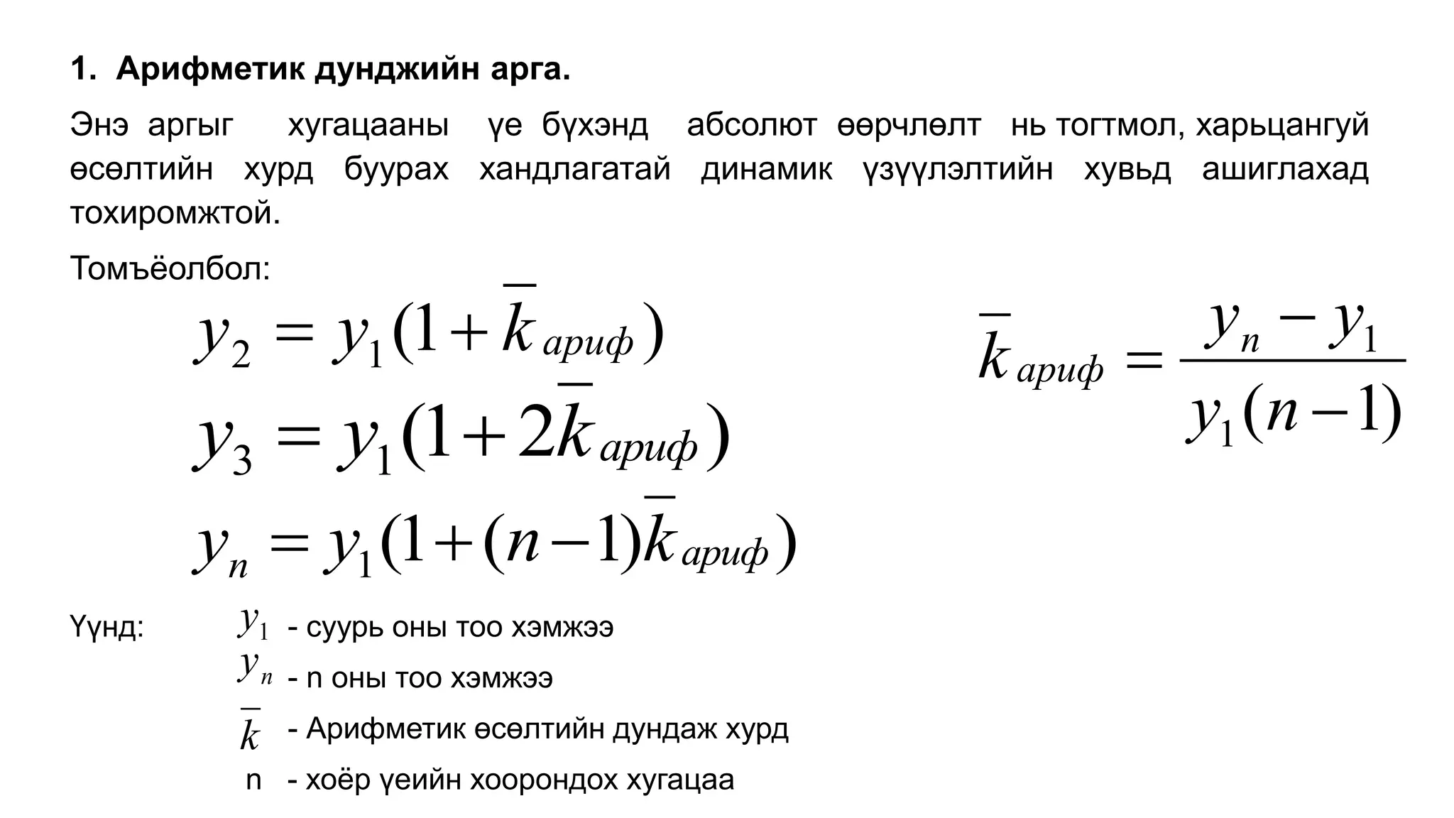
1. Арифметик дунджийнарга.
Энэ аргыг хугацааны үе бүхэнд абсолют өөрчлөлт нь тогтмол, харьцангуй
өсөлтийн хурд буурах хандлагатай динамик үзүүлэлтийн хувьд ашиглахад
тохиромжтой.
Томъёолбол:
Үүнд: - суурь оны тоо хэмжээ
- n оны тоо хэмжээ
- Арифметик өсөлтийн дундаж хурд
n - хоёр үеийн хоорондох хугацаа
)
1
(
1
2 ариф
k
y
y
)
2
1
(
1
3 ариф
k
y
y
)
)
1
(
1
(
1 ариф
n k
n
y
y
1
y
n
y
k
)
1
(
1
1
n
y
y
y
k n
ариф
19.
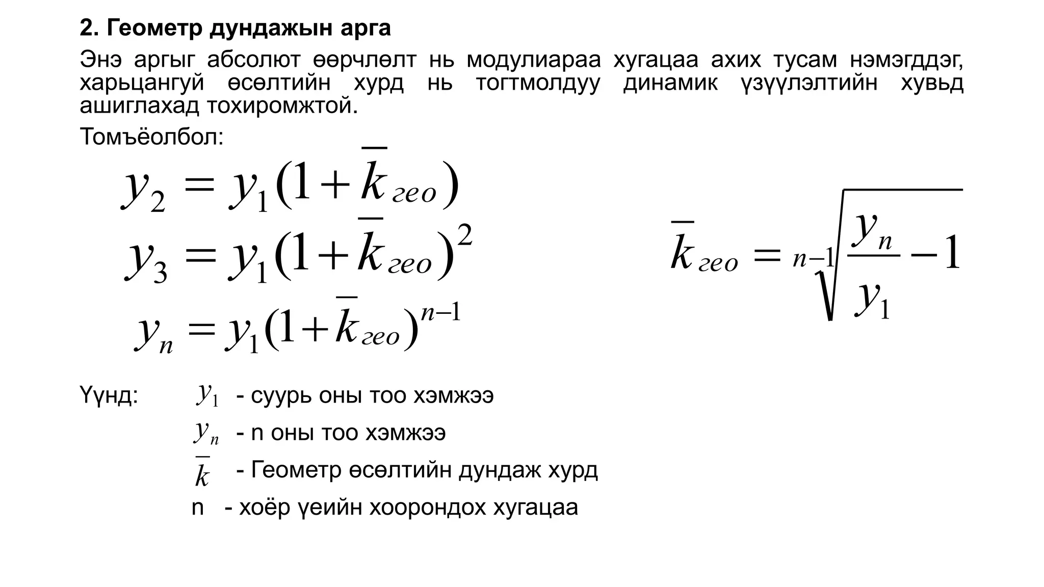
2. Геометр дундажынарга
Энэ аргыг абсолют өөрчлөлт нь модулиараа хугацаа ахих тусам нэмэгддэг,
харьцангуй өсөлтийн хурд нь тогтмолдуу динамик үзүүлэлтийн хувьд
ашиглахад тохиромжтой.
Томъёолбол:
Үүнд: - суурь оны тоо хэмжээ
- n оны тоо хэмжээ
- Геометр өсөлтийн дундаж хурд
n - хоёр үеийн хоорондох хугацаа
)
1
(
1
2 гео
k
y
y
2
1
3 )
1
( гео
k
y
y
1
1 )
1
(
n
гео
n k
y
y
1
y
n
y
k
1
1
1
n
n
гео
y
y
k
20.
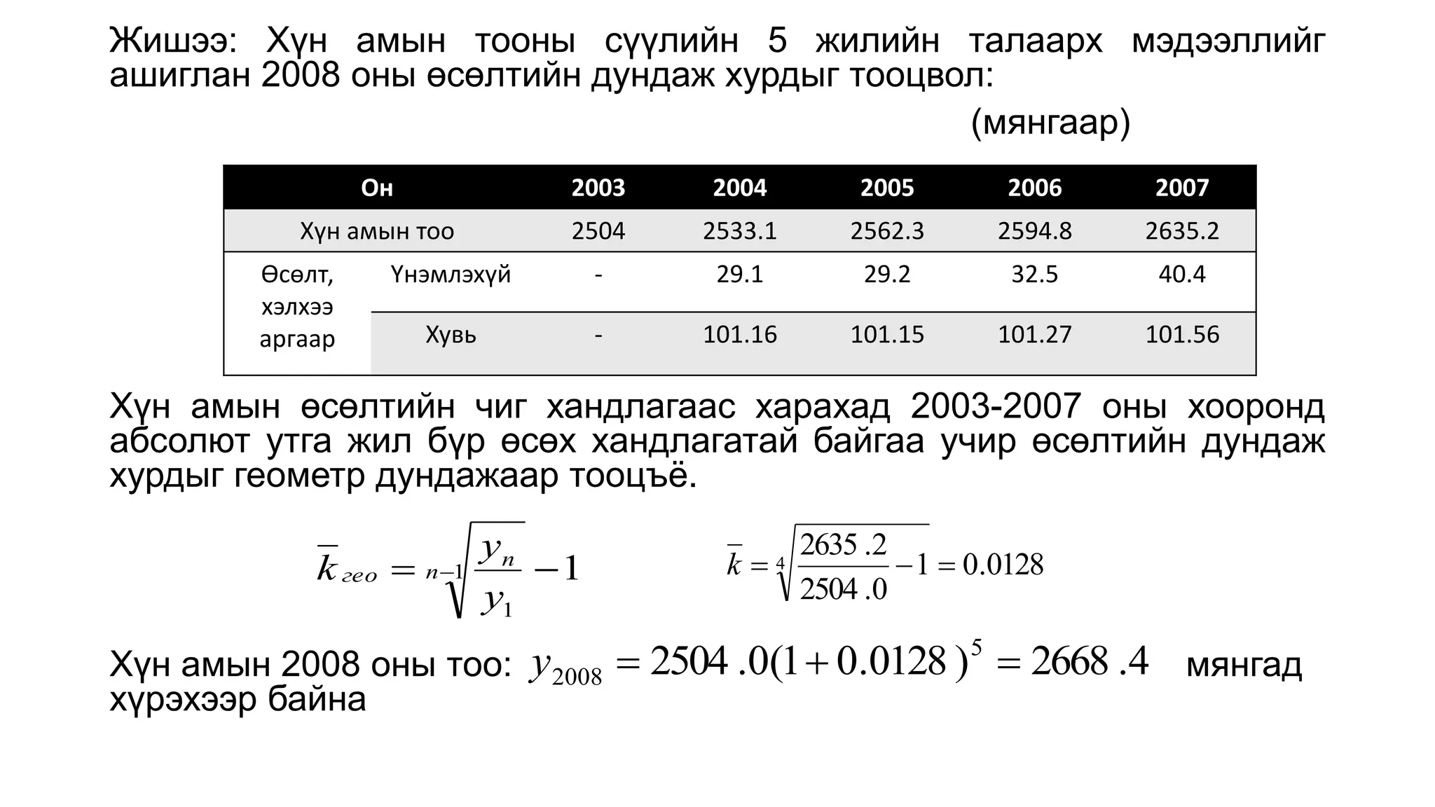
Жишээ: Хүн амынтооны сүүлийн 5 жилийн талаарх мэдээллийг
ашиглан 2008 оны өсөлтийн дундаж хурдыг тооцвол:
(мянгаар)
Хүн амын өсөлтийн чиг хандлагаас харахад 2003-2007 оны хооронд
абсолют утга жил бүр өсөх хандлагатай байгаа учир өсөлтийн дундаж
хурдыг геометр дундажаар тооцъё.
Хүн амын 2008 оны тоо: мянгад
хүрэхээр байна
Он 2003 2004 2005 2006 2007
Хүн амын тоо 2504 2533.1 2562.3 2594.8 2635.2
Өсөлт,
хэлхээ
аргаар
Үнэмлэхүй - 29.1 29.2 32.5 40.4
Хувь - 101.16 101.15 101.27 101.56
0128
.
0
1
0
.
2504
2
.
2635
4
k
4
.
2668
)
0128
.
0
1
(
0
.
2504 5
2008
y
1
1
1
n
n
гео
y
y
k
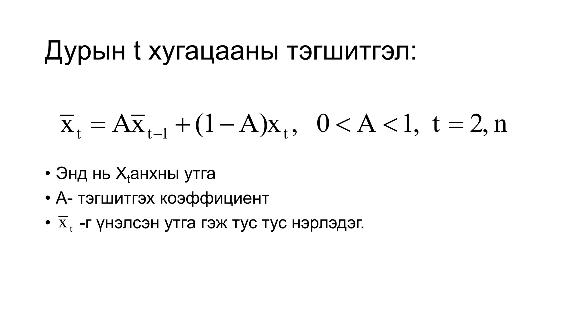
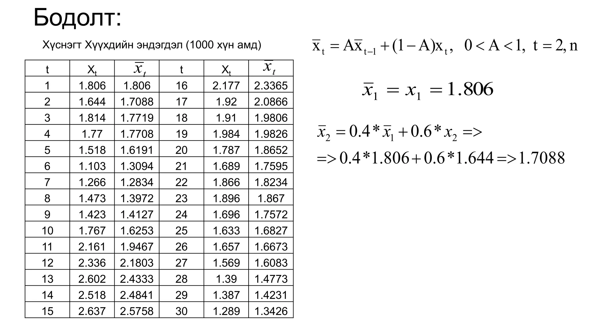
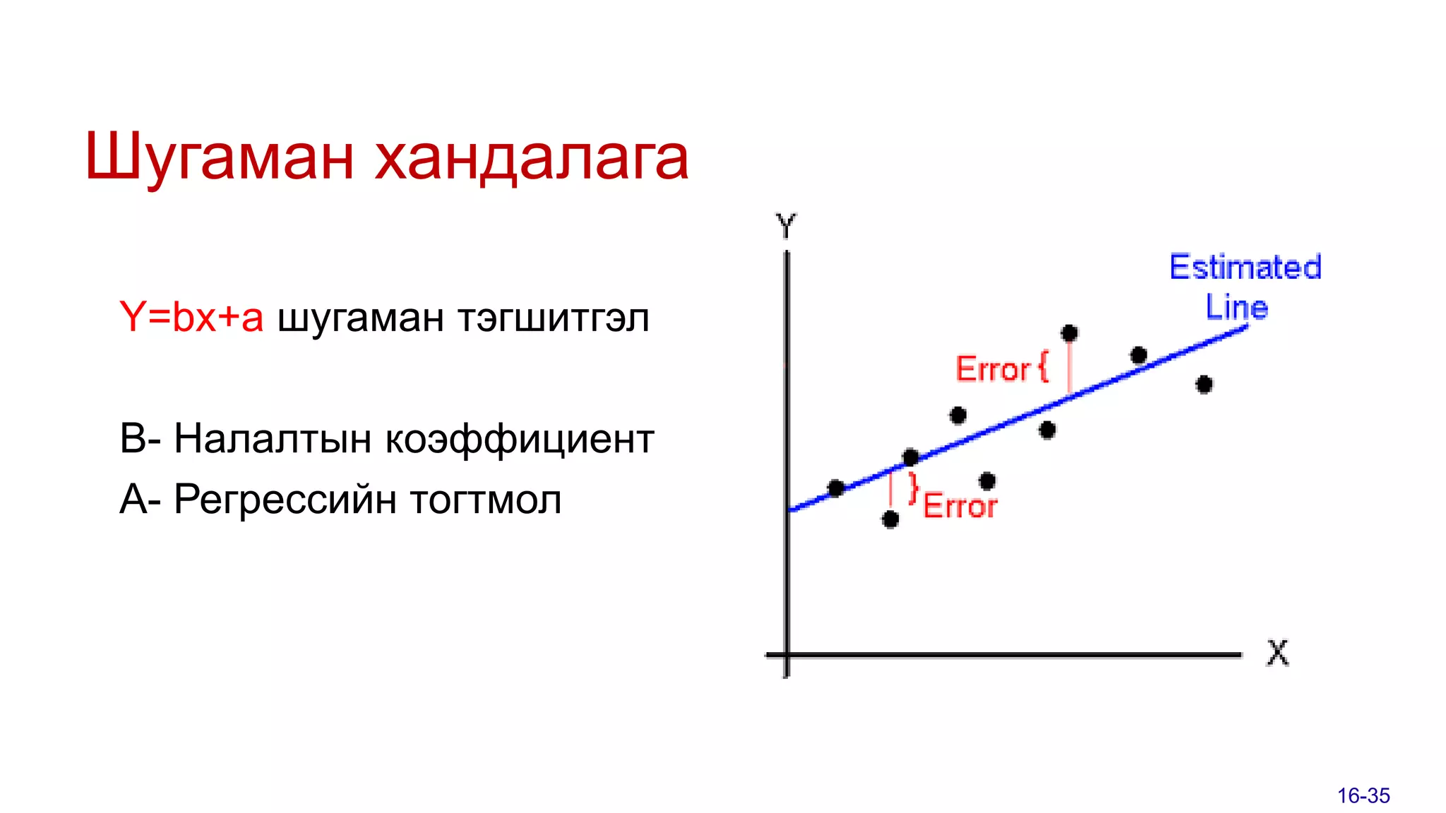
Дурын t хугацаанытэгшитгэл:
n
2,
t
1,
A
0
,
A)x
(1
x
A
x t
1
t
t
• Энд нь Xtанхны утга
• А- тэгшитгэх коэффициент
• -г үнэлсэн утга гэж тус тус нэрлэдэг.
t
x
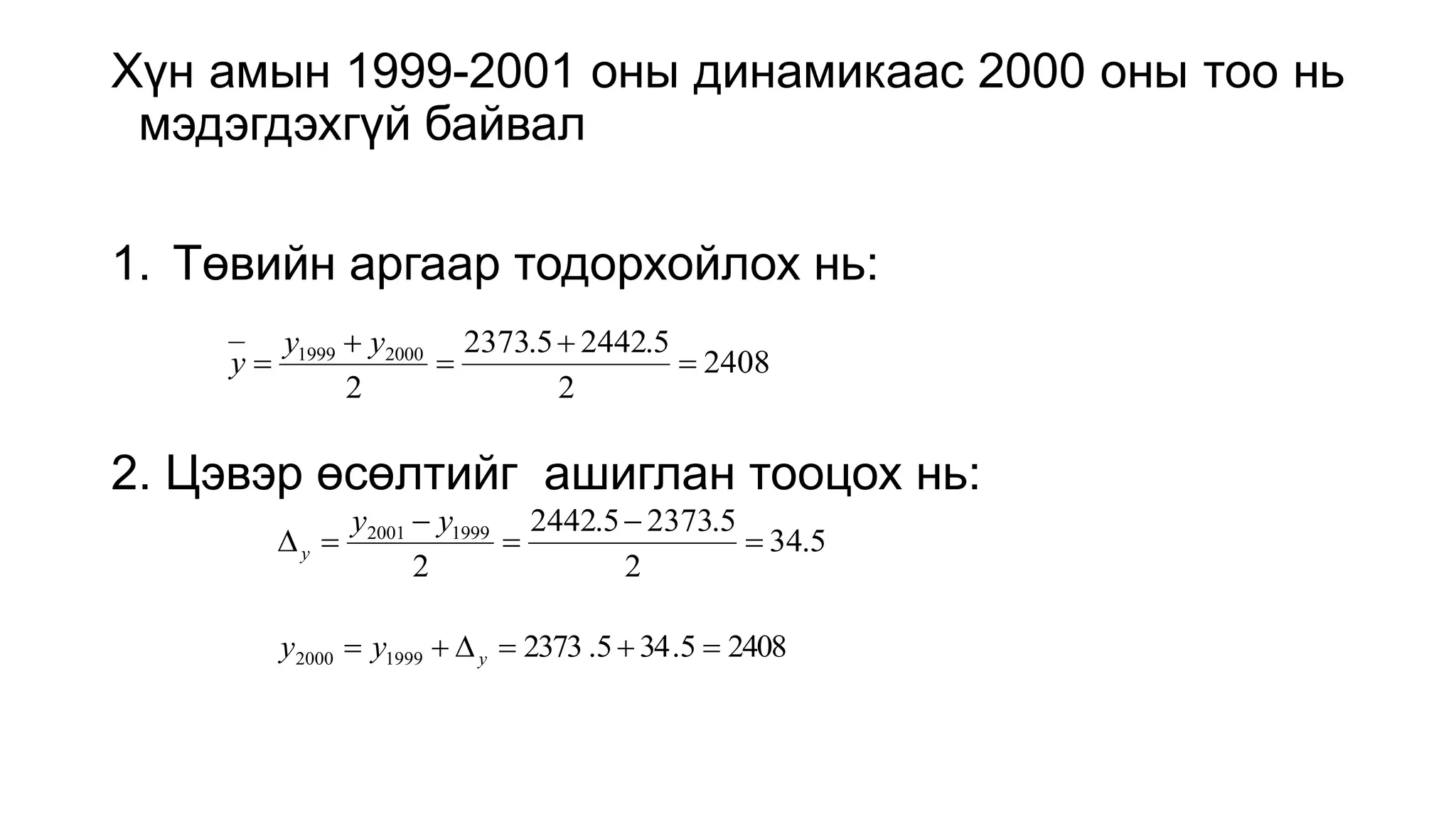
Хүн амын 1999-2001оны динамикаас 2000 оны тоо нь
мэдэгдэхгүй байвал
1. Төвийн аргаар тодорхойлох нь:
2. Цэвэр өсөлтийг ашиглан тооцох нь:
2408
2
5
.
2442
5
.
2373
2
2000
1999
y
y
y
5
.
34
2
5
.
2373
5
.
2442
2
1999
2001
y
y
y
2408
5
.
34
5
.
2373
1999
2000
y
y
y
28.
Абсолют өсөлт
Абсолют өсөлтнь өмнөх хугацааны түвшнөөс ямар
хэмжээгээр өссөн эсвэл буурсан болохыг харууладг
үзүүлэлт юм. Энэ үзүүлэлт нь зэрэгцээ хоёр түвшингийн
ялгаврын модулиар илэрхийлэгдэнэ.
1
t
t
t x
x
Δ
29.
Дундаж абсолют өсөлт
Дундажабсолют өсөлт нь тухайн хугацааны цуваа жил
болгон дундажаар ямар хэмжээгээр өсөх, дундажаар ямар
хэмжээгээр буурахыг илэрхийлдэг.
1
n
x
x
Δ
1
n
30.
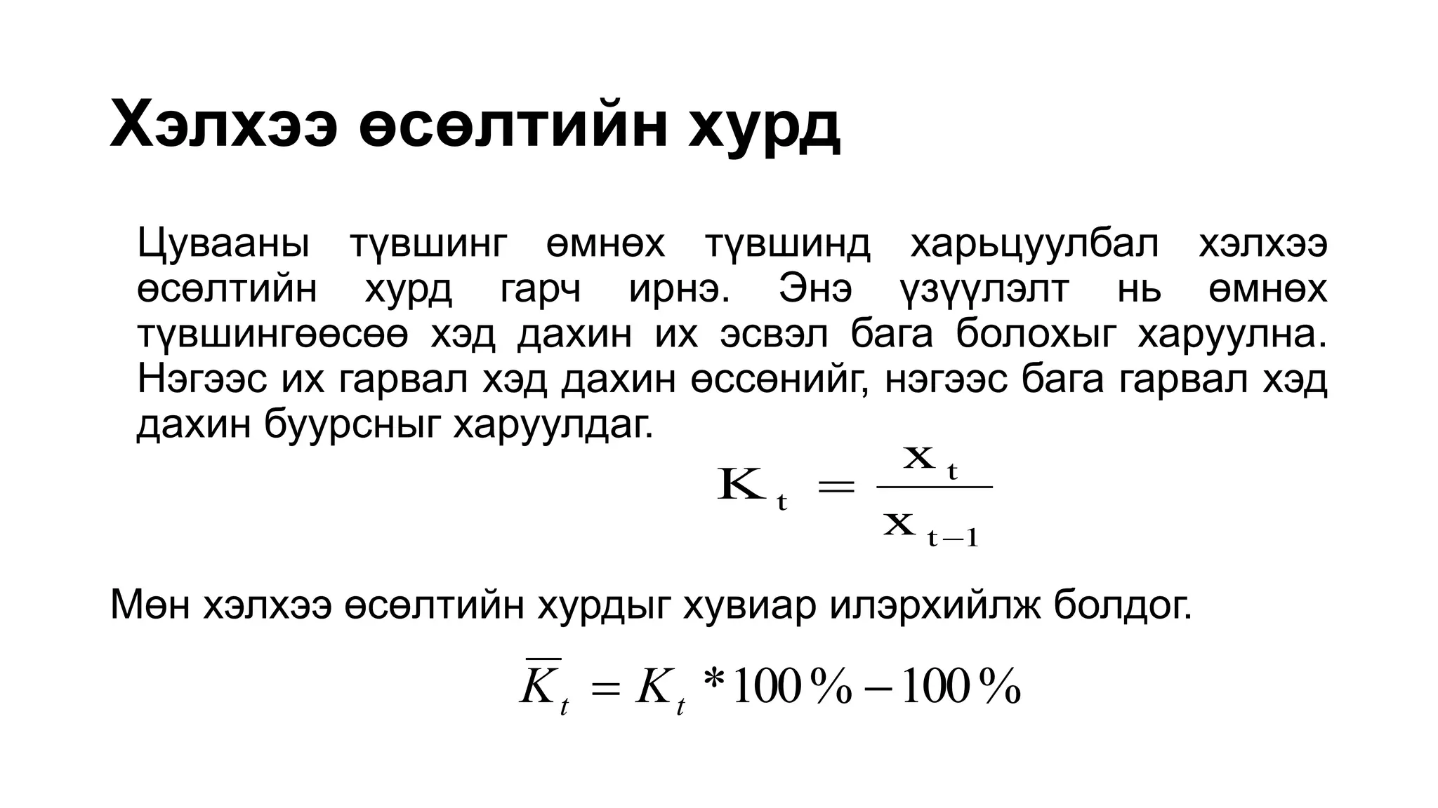
Хэлхээ өсөлтийн хурд
Цуваанытүвшинг өмнөх түвшинд харьцуулбал хэлхээ
өсөлтийн хурд гарч ирнэ. Энэ үзүүлэлт нь өмнөх
түвшингөөсөө хэд дахин их эсвэл бага болохыг харуулна.
Нэгээс их гарвал хэд дахин өссөнийг, нэгээс бага гарвал хэд
дахин буурсныг харуулдаг.
Мөн хэлхээ өсөлтийн хурдыг хувиар илэрхийлж болдог.
1
t
t
t
x
x
K
%
100
%
100
*
t
t K
K
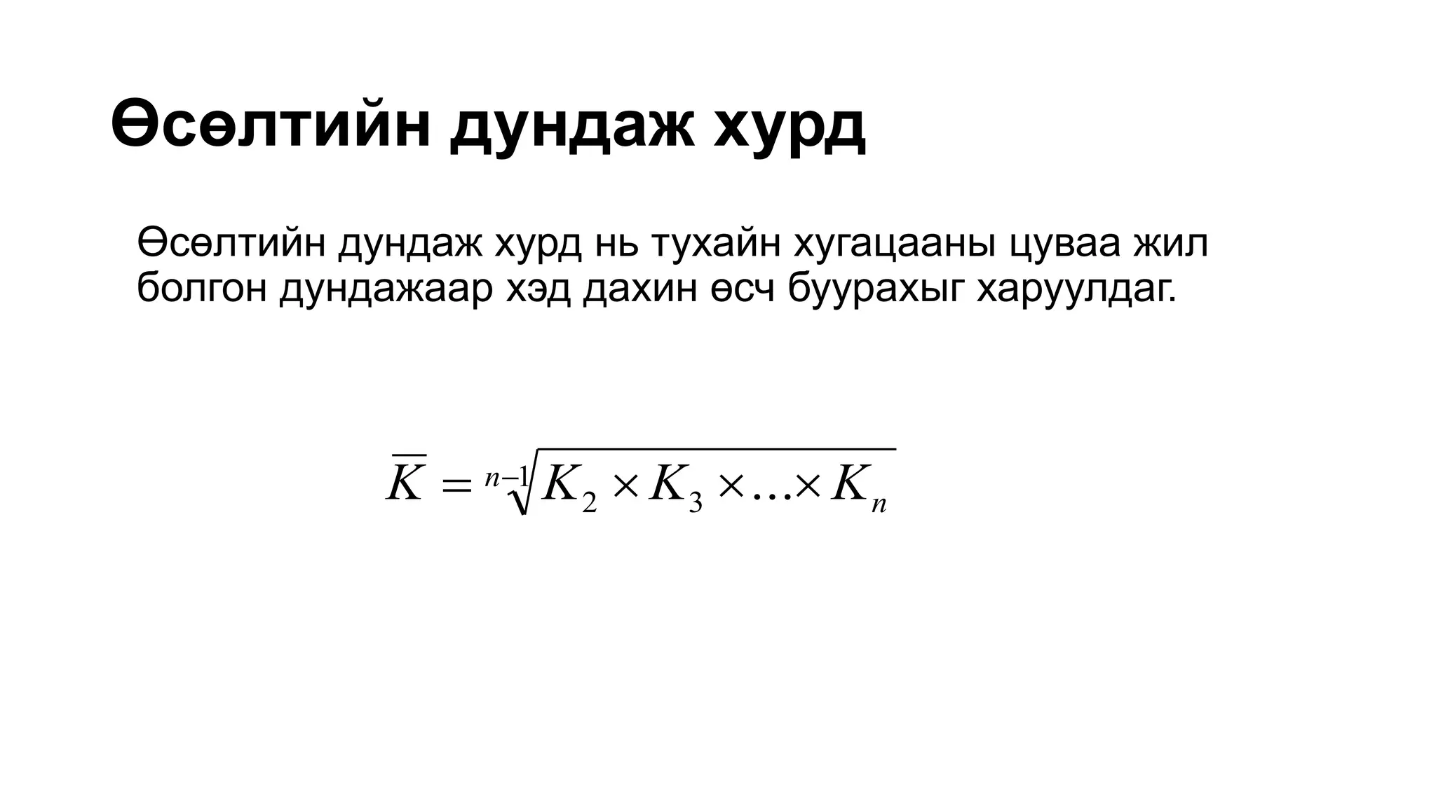
Өсөлтийн дундаж хурд
Өсөлтийндундаж хурд нь тухайн хугацааны цуваа жил
болгон дундажаар хэд дахин өсч буурахыг харуулдаг.
1
3
2 ...
n
n
K
K
K
K
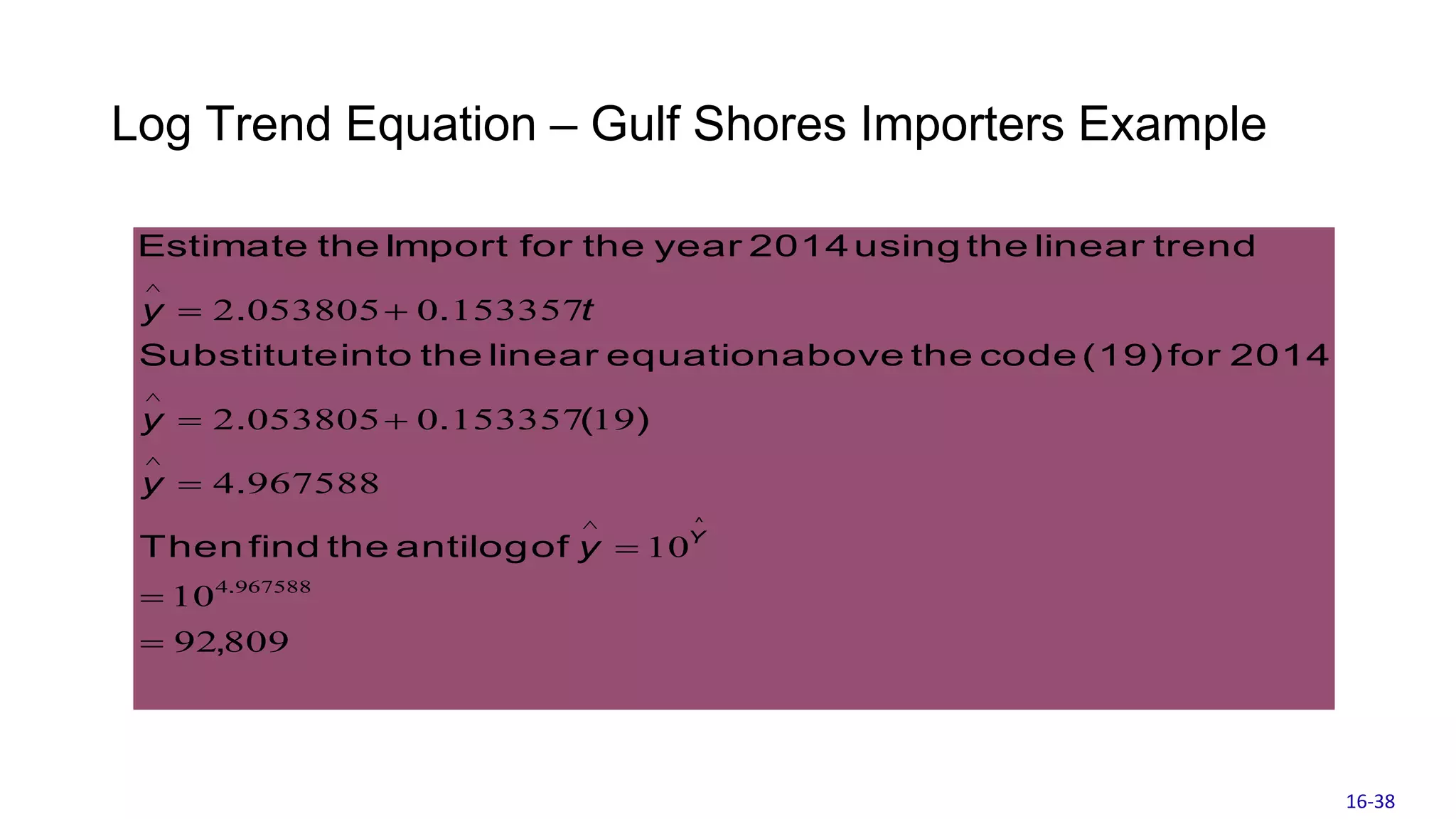
Log Trend Equation– Gulf Shores Importers Example
809
92
10
10
967588
4
19
153357
0
053805
2
153357
0
053805
2
967588
4
,
of
antilog
the
find
Then
.
)
(
.
.
2014
for
(19)
code
the
above
equation
linear
the
into
Substitute
.
.
trend
linear
the
using
2014
year
the
for
Import
the
Estimate
.
^
Y
y
y
y
t
y
16-38
39.
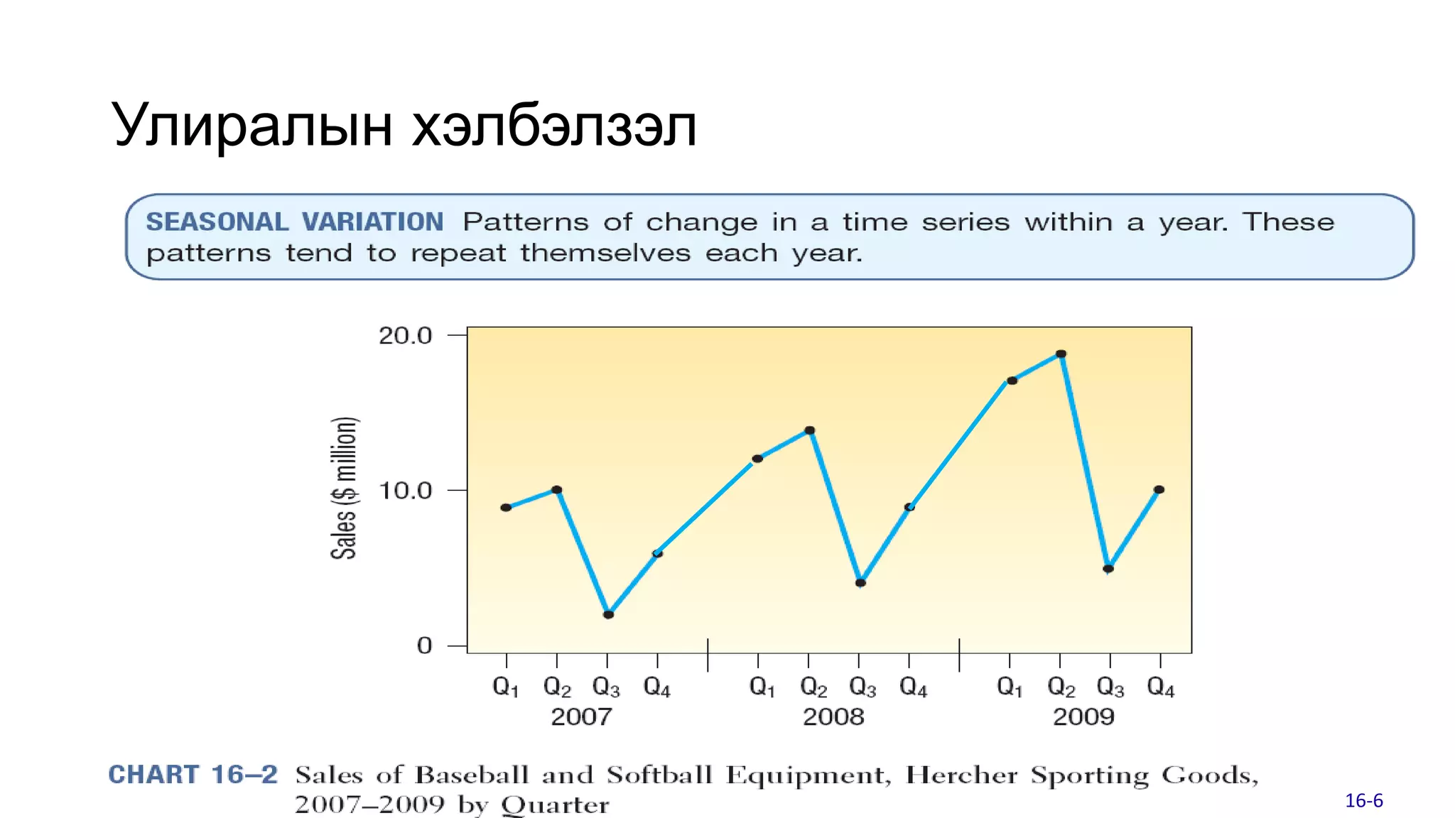
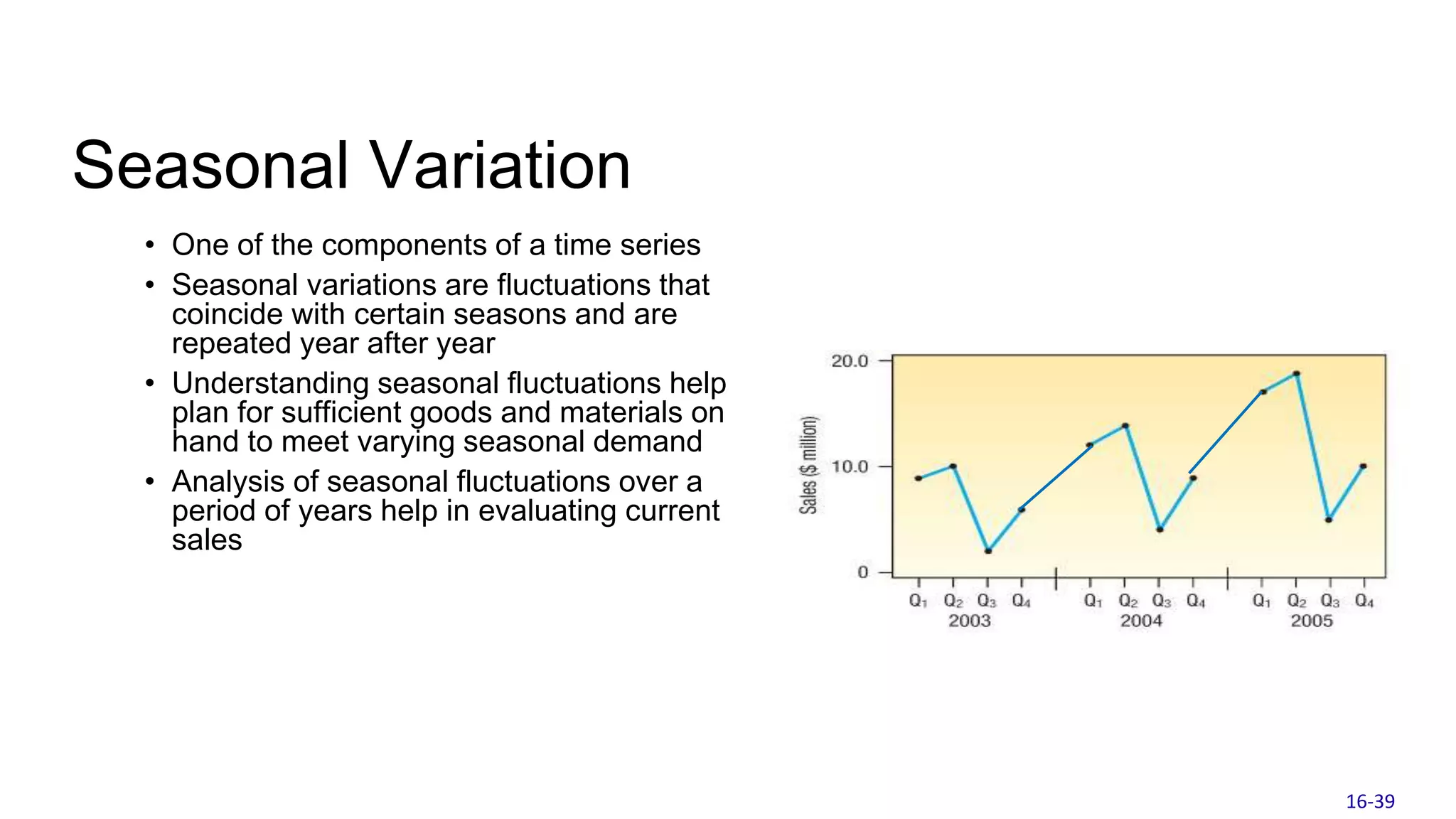
Seasonal Variation
• Oneof the components of a time series
• Seasonal variations are fluctuations that
coincide with certain seasons and are
repeated year after year
• Understanding seasonal fluctuations help
plan for sufficient goods and materials on
hand to meet varying seasonal demand
• Analysis of seasonal fluctuations over a
period of years help in evaluating current
sales
16-39
40.
Seasonal Index
• Anumber, usually expressed in percent, that expresses the
relative value of a season with respect to the average for the year
(100%)
• Ratio-to-moving-average method
• The method most commonly used to compute the typical seasonal pattern
• It eliminates the trend (T), cyclical (C), and irregular (I) components from
the time series
16-40
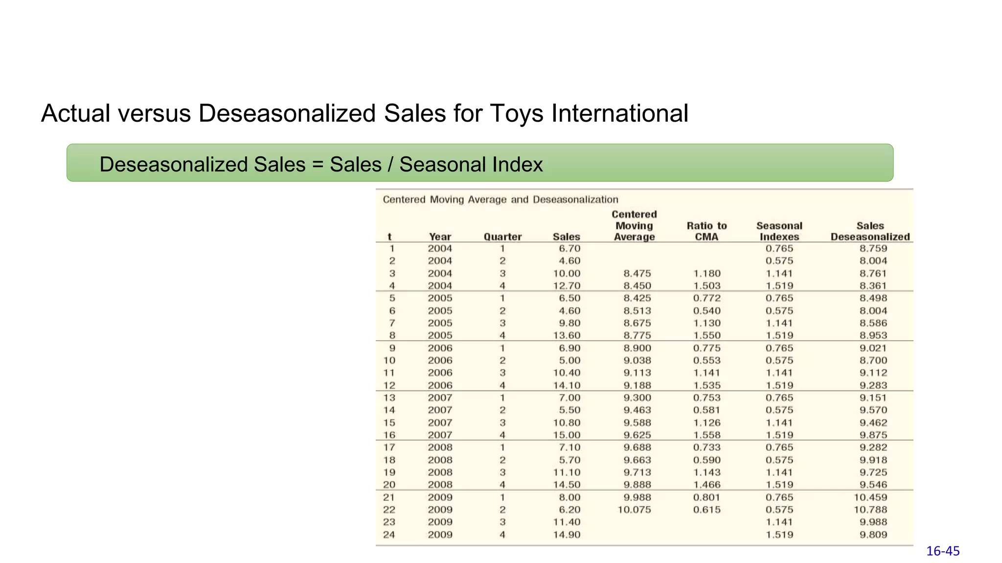
41.
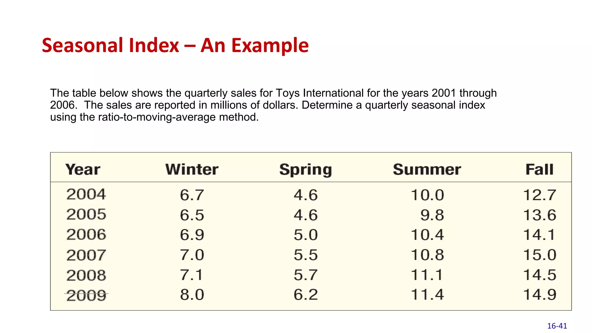
The table belowshows the quarterly sales for Toys International for the years 2001 through
2006. The sales are reported in millions of dollars. Determine a quarterly seasonal index
using the ratio-to-moving-average method.
Seasonal Index – An Example
16-41
42.
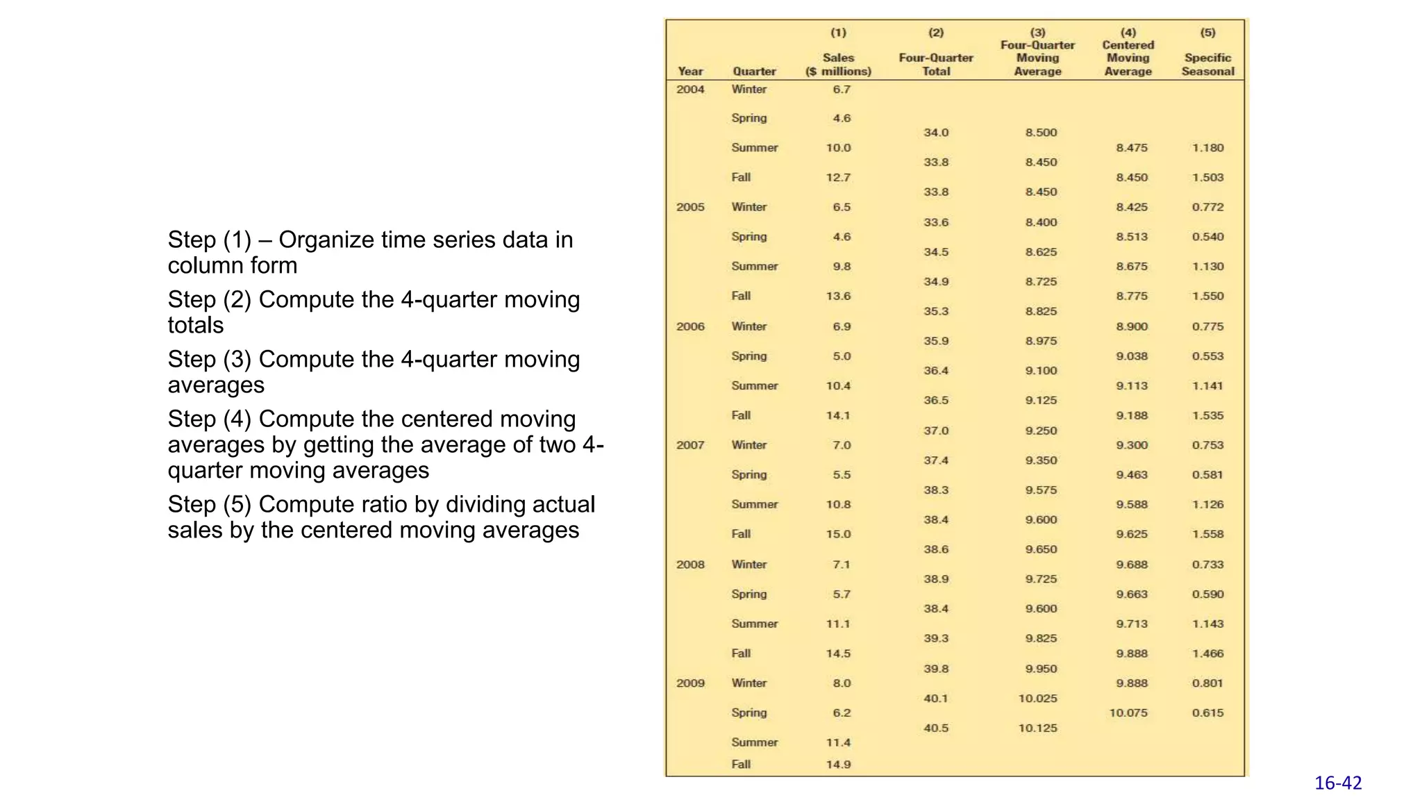
Step (1) –Organize time series data in
column form
Step (2) Compute the 4-quarter moving
totals
Step (3) Compute the 4-quarter moving
averages
Step (4) Compute the centered moving
averages by getting the average of two 4-
quarter moving averages
Step (5) Compute ratio by dividing actual
sales by the centered moving averages
16-42
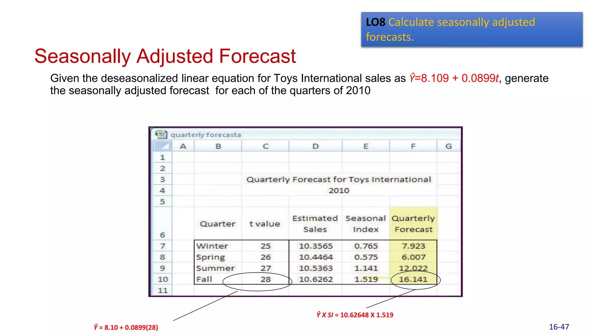
Seasonally Adjusted Forecast
Giventhe deseasonalized linear equation for Toys International sales as Ŷ=8.109 + 0.0899t, generate
the seasonally adjusted forecast for each of the quarters of 2010
Ŷ = 8.10 + 0.0899(28)
Ŷ X SI = 10.62648 X 1.519
LO8 Calculate seasonally adjusted
forecasts.
16-47
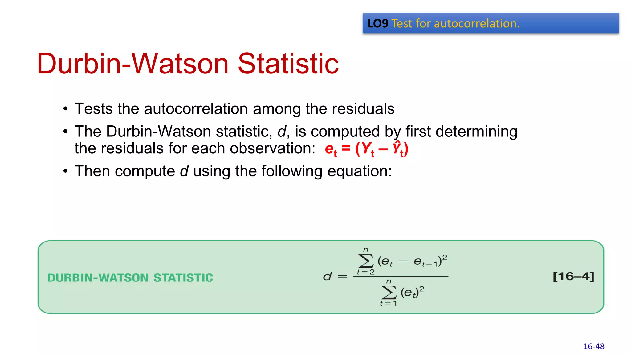
48.
Durbin-Watson Statistic
• Teststhe autocorrelation among the residuals
• The Durbin-Watson statistic, d, is computed by first determining
the residuals for each observation: et = (Yt – Ŷt)
• Then compute d using the following equation:
LO9 Test for autocorrelation.
16-48
49.
Durbin-Watson Test forAutocorrelation – Interpretation of the
Statistic
• Range of d is 0 to 4
d = 2 No autocorrelation
d close to 0 Positive autocorrelation
d beyond 2 Negative autocorrelation
• Hypothesis Test:
H0: No residual correlation (ρ = 0)
H1: Positive residual correlation (ρ > 0)
• Critical values for d are found in Appendix B.10 using
• α - significance level
• n – sample size
• K – the number of predictor variables
LO9
16-49
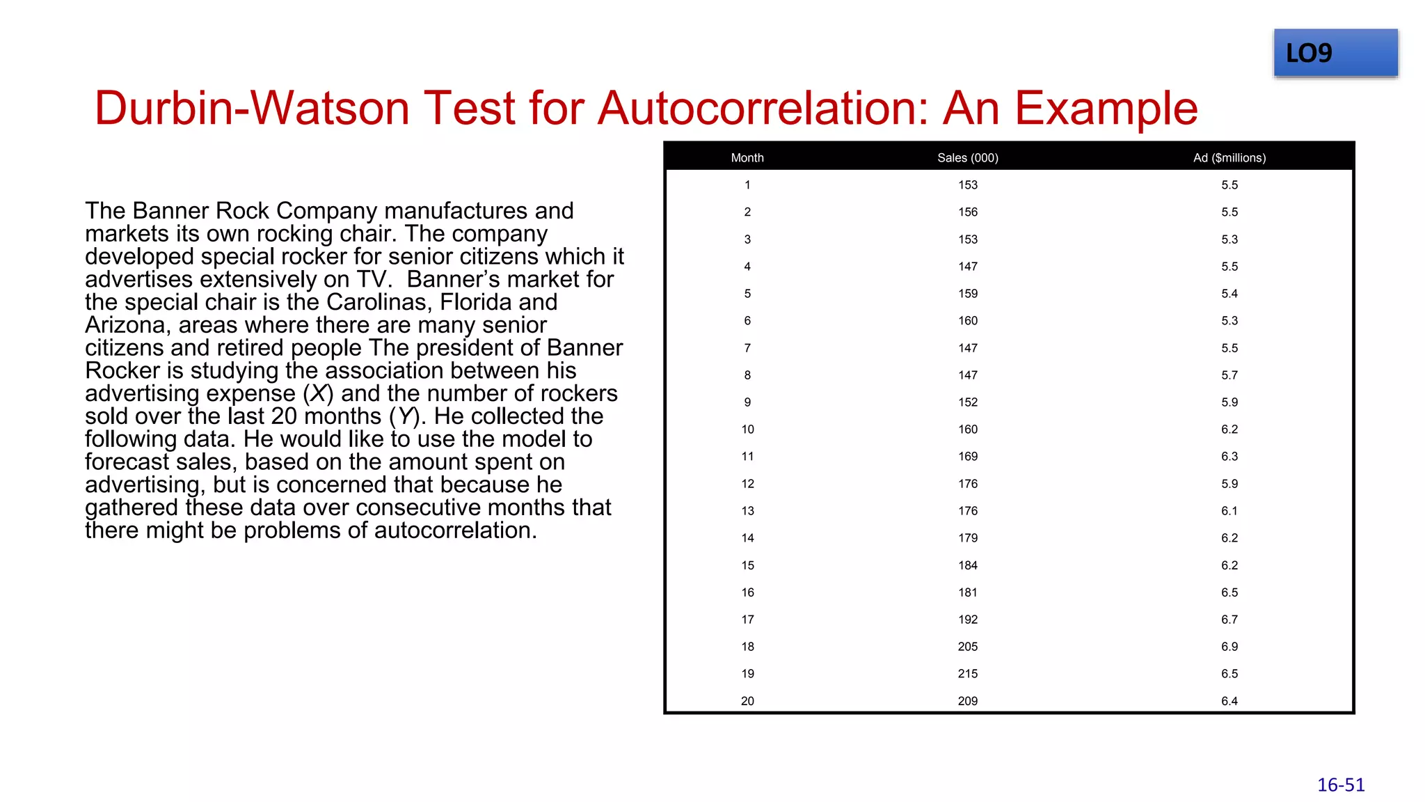
Durbin-Watson Test forAutocorrelation: An Example
The Banner Rock Company manufactures and
markets its own rocking chair. The company
developed special rocker for senior citizens which it
advertises extensively on TV. Banner’s market for
the special chair is the Carolinas, Florida and
Arizona, areas where there are many senior
citizens and retired people The president of Banner
Rocker is studying the association between his
advertising expense (X) and the number of rockers
sold over the last 20 months (Y). He collected the
following data. He would like to use the model to
forecast sales, based on the amount spent on
advertising, but is concerned that because he
gathered these data over consecutive months that
there might be problems of autocorrelation.
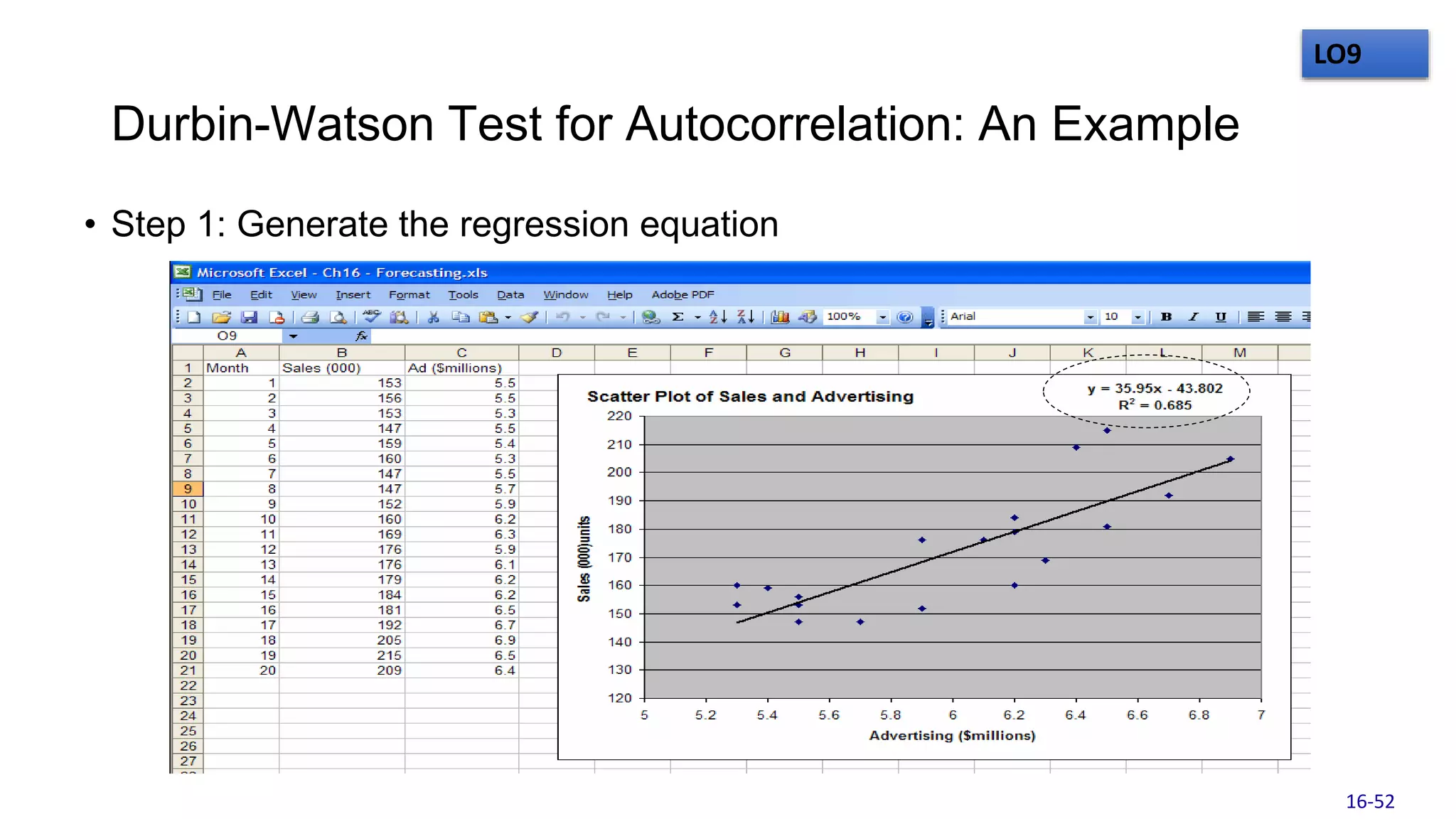
Month Sales (000) Ad ($millions)
1 153 5.5
2 156 5.5
3 153 5.3
4 147 5.5
5 159 5.4
6 160 5.3
7 147 5.5
8 147 5.7
9 152 5.9
10 160 6.2
11 169 6.3
12 176 5.9
13 176 6.1
14 179 6.2
15 184 6.2
16 181 6.5
17 192 6.7
18 205 6.9
19 215 6.5
20 209 6.4
LO9
16-51
52.
Durbin-Watson Test forAutocorrelation: An Example
• Step 1: Generate the regression equation
LO9
16-52
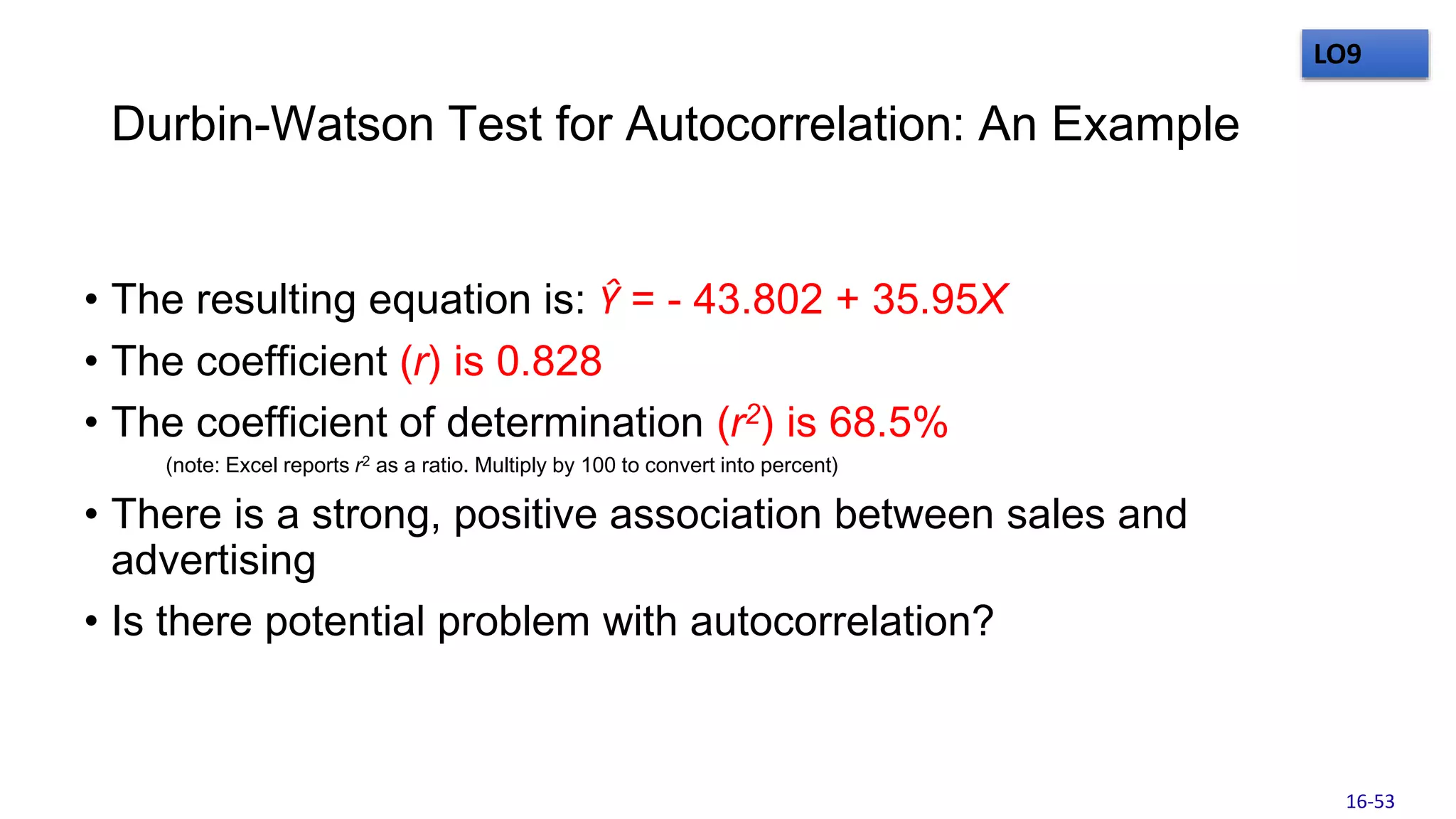
53.
Durbin-Watson Test forAutocorrelation: An Example
• The resulting equation is: Ŷ = - 43.802 + 35.95X
• The coefficient (r) is 0.828
• The coefficient of determination (r2) is 68.5%
(note: Excel reports r2 as a ratio. Multiply by 100 to convert into percent)
• There is a strong, positive association between sales and
advertising
• Is there potential problem with autocorrelation?
LO9
16-53
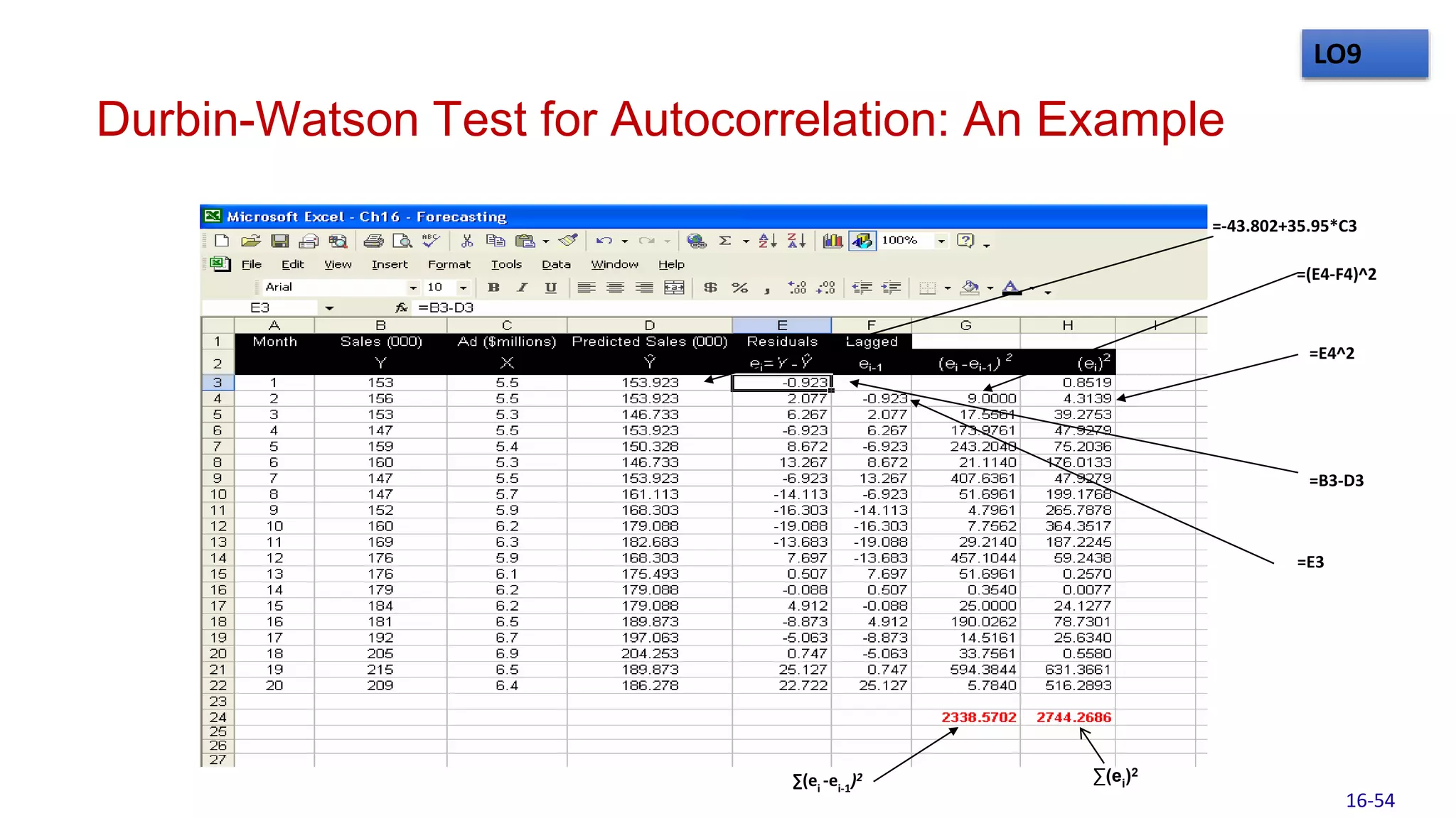
54.
Durbin-Watson Test forAutocorrelation: An Example
∑(ei -ei-1)2 ∑(ei)2
=E4^2
=(E4-F4)^2
=-43.802+35.95*C3
=B3-D3
=E3
LO9
16-54
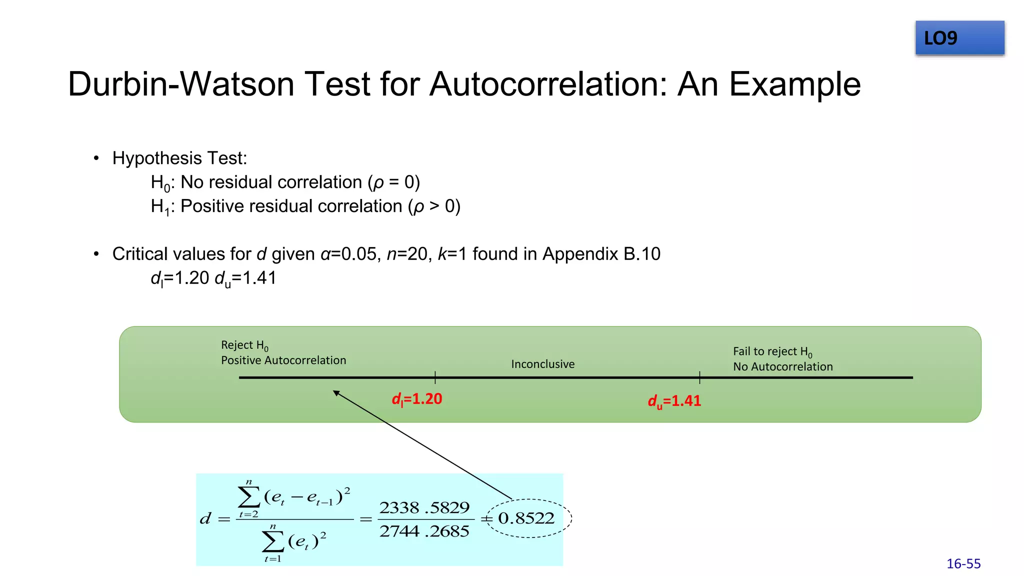
55.
Durbin-Watson Test forAutocorrelation: An Example
• Hypothesis Test:
H0: No residual correlation (ρ = 0)
H1: Positive residual correlation (ρ > 0)
• Critical values for d given α=0.05, n=20, k=1 found in Appendix B.10
dl=1.20 du=1.41
8522
.
0
2685
.
2744
5829
.
2338
)
(
)
(
1
2
2
2
1
n
t
t
n
t
t
t
e
e
e
d
dl=1.20 du=1.41
Reject H0
Positive Autocorrelation Inconclusive
Fail to reject H0
No Autocorrelation
LO9
16-55