Spectrograms allow phoneticians to visualize how the frequency spectrum of speech sounds changes over time. They plot frequency on the vertical axis, time on the horizontal axis, and intensity as color. Narrowband spectrograms provide detailed frequency information while wideband spectrograms precisely show timing. Common speech sounds like vowels, consonants, and transitions between them exhibit characteristic patterns. Reading spectrograms is essential for instrumental phonetics research.

1. Spectrograms
An essential tool for instrumental phonetics

2. Voice Spectra and Spectrograms
• Recall that power spectra allow us to see the component frequencies and amplitudes
that make up a complex wave.
• Spectrograms are a way of viewing hundreds of sequential power spectra, so we can
see how the spectrum of a speech signal changes over time.
– This is done by turning the spectrum sideways, reducing each bar on the spectrum to a
dot, and using the color of the dot to symbolize the height of the bar (i.e., the amplitude or
intensity of the component frequency).
2

3. Building a Spectrogram
1. Power spectrum
amplitudes are
represented as different
shades of grey (taller =
darker)
2. Spectrum is rotated and
collapsed to 1-dimension.
3. Hundreds of spectra are
arrayed side by side,
allowing us to see
changes in formant
frequencies over time.
3

4. Reading a Spectrogram
• A spectrogram plots three variables:
– The horizontal axis is time, usually
measured in milliseconds.
– The vertical axis is frequency (Hz).
– The third variable, intensity, is represented
by the color of each point that is plotted.
• The dark bands show the formants of the
voiced sounds.
– The first three formants vary depending on
the shape of the vocal tract and are
important for understanding the speech
signal.
frequency
time (ms)
4

5. Narrowband Spectrograms
• When calculating the frequency components that make up the speech signal, it is necessary
to take a chunk of time to figure out the frequency of the wave.
• Narrowband spectrograms show calculations based on longer chunks of time, which allows
more accurate calculation of the frequencies making up the signal and can reveal individual
harmonics of the signal.
– Because the chunks of time are longer, narrowband spectrograms are less precise about when a
given speech event happened (e.g., a release burst or the onset of voicing). This lack of precision in
the temporal dimension is called time smear.
– Because of their detailed frequency information, narrowband spectrograms are useful for
investigating changes in pitch, tone, and intonation.
5

6. Narrowband Spectrograms
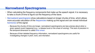
• [ɑbɑ]
– Frequency range: 0 – 5000 Hz; duration: ≈0.75 s
– Window size: 0.05 s
Individual
harmonics
6

7. Wideband Spectrograms
• Wideband spectrograms show calculations based on short chunks of time, which allows
accurate measurement of event timing at the expense of detailed frequency information.
Wideband spectrograms are vertically striated; each vertical striation shows an individual
vibration of the vocal folds.
– Remember that formants are broad peaks of intensity that range over several neighboring
frequencies. Since the wideband spectrograms “smear together” neighboring frequencies, this
actually helps us to see the formants more clearly.
– Vowel quality, place of articulation, and other segmental features are all aspects of the filter and thus
cause broad-frequency changes to the signal. Thus they are best viewed using wideband
spectrograms.
– Because of their accurate timing calculations, wideband spectrograms are also useful for measuring
VOT, vowel duration, and other time-based characteristics of speech.
7

8. Wideband Spectrograms
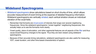
• [ɑbɑ]
– Frequency range: 0 – 5000 Hz; duration: ≈0.75 s
– Window size: 0.01 s
Formants
vertical striations
8

9. Reading a Spectrogram: Voicing
• Voiced sounds have a dark band very close to the bottom of the spectrogram,
corresponding to the fundamental frequency of the speaker’s voice.
– Many “voiced” consonants are allophonically devoiced, so the absence of a voicing band
does not guarantee that the sound is a voiceless phoneme.
9

10. Reading a Spectrogram: Voicing
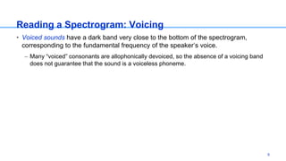
• [ɑzɑ]
– Frequency range: 0 – 5000 Hz; duration: ≈0.75 s
Voicing band
10

11. Reading a Spectrogram: Voicing
• [ɑsɑ]
– Frequency range: 0 – 5000 Hz; duration: ≈0.75 s
No voicing band
11

12. Reading a Spectrogram: Approximants
• Vowels and approximants show vertical striations in wideband spectrograms, and
clear dark formant bands.
– Vowels are identified on a spectrogram primarily by the values of their F1 and F2 formants.
– Approximants involve constriction comparable to that of a high vowel, and so tend to have
fairly low F1 values. Approximants can often be distinguished by the movement of their F2
and F3 formants.
12

13. Reading a Spectrogram: Approximants
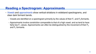
• [ɑlɑ]
– Frequency range: 0 – 5000 Hz; duration: ≈0.75 s
Formants
low F1 value for the approximant [ l]
13

14. Reading a Spectrogram: Oral Stops
• Oral stops involve complete stoppage of airflow and thus show up as a “gap” in the
spectrogram.
– The formant transitions of the voiced sounds before or after a stop are the best way to
determine the stop’s place of articulation.
– The release burst of a stop may be continuous with a following voiced sound, or may stand
alone at the end of a word as a brief vertical band of high energy. The distribution of that
energy can also provide clues to the place of articulation of the stop.
14

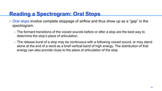
15. Reading a Spectrogram: Oral Stops
• [ɑpɑ]
– Frequency range: 0 – 5000 Hz; duration: ≈0.75 s
period of closure aspiration noise
release burst
15

16. Reading a Spectrogram: Nasal Stops
• Nasal stops allow continuation of airflow and show formant structure much like
vowels.
– Like oral stops, nasal place of articulation is most easily determined by the formant
transitions of the surrounding vowels.
– Unlike vowels, nasals typically show “zeroes” (white areas) between the lower formants.
– Nasals can be distinguished from vowels by a much lower amplitude in the waveform (not
the spectrogram).
16

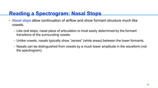
17. Reading a Spectrogram: Nasal Stops
• [ɑnɑ]
– Frequency range: 0 – 5000 Hz; duration: ≈0.75 s
“zeroes”
17

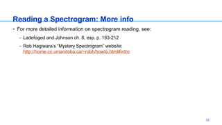
18. Reading a Spectrogram: Nasal Stops
• [ɑnɑ]
lower amplitude
18

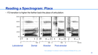
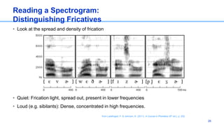
19. Reading a Spectrogram: Fricatives
• Fricatives are characterized by fairly high energy (darker color) especially in the
higher frequencies, and (usually) a lack of formant bands.
– [h] often does show formant bands. This is because [h] generates turbulence in the same
place that voicing originates (the glottis), so the turbulence of [h] is subject to the same
filter that vowels are (namely, the entire vocal tract). The spectrum of [h] can vary widely
depending on the following vowel.
19

20. Reading a Spectrogram: Fricatives
• [ɑʃɑ]
– Frequency range: 0 – 10,000 Hz; duration: ≈0.75 s
high energy in the higher frequencies
20

21. Reading a Spectrogram: Fricatives
• [ɑhɑ]
– Frequency range: 0 – 10,000 Hz; duration: ≈0.75 s
formant bands visible through the [h]
21

22. Reading a Spectrogram: More info
• For more detailed information on spectrogram reading, see:
– Ladefoged and Johnson ch. 8, esp. p. 193-212
– Rob Hagiwara’s “Mystery Spectrogram” website:
http://home.cc.umanitoba.ca/~robh/howto.html#intro
22

23. Reading a Spectrogram: Vowels
from Ladefoged, P. & Johnson, K. (2011). A Course in Phonetics (6th ed.), p. 194.
23

24. Formant Transitions:
Cues to Place of Articulation
from Johnson, K. (2003). Acoustic & Auditory Phonetics (2nd ed.). Malden, MA: Blackwell.
24

25. Reading a Spectrogram: Place
• F2 transition is higher the farther back the place of articulation:
Labiodental Dental Alveolar Post-alveolar
25
from Ladefoged, P. & Johnson, K. (2011). A Course in Phonetics (6th ed.), p. 201.

26. Reading a Spectrogram:
Distinguishing Fricatives
• Look at the spread and density of frication
• Quiet: Frication light, spread out, present in lower frequencies
• Loud (e.g. sibilants): Dense, concentrated in high frequencies.
26
from Ladefoged, P. & Johnson, K. (2011). A Course in Phonetics (6th ed.), p. 202.

27. Reading a Spectrogram:
Distinguishing Approximants
• Approximants flow smoothly into vowels
27
from Ladefoged, P. & Johnson, K. (2011). A Course in Phonetics (6th ed.), p. 202.
• [l] – dip in F2, slight rise in F3
• [ɹ] – central F2, scoop in F3
• [w] – like high back vowel [u/ʊ]
• [j] – like high front vowel [i/ɪ]

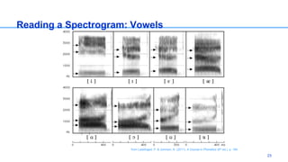
28. Spectrogram Examples: [ɹ]
• Scoop shape to F3 • F2 central (between front & back vowels)
28
1800 Hz
1500 Hz
500 Hz
[ m ɛ ɹ i ] [ k ɑ ɹ ]